1  Importing and Handling Genomic Data

Session Presenters

Required packages

library(dartRverse)
library(dartR.sexlinked)

Introduction

SNPs, or single nucleotide polymorphisms, are single base pair mutations at a nuclear locus (Figure 2). That nuclear locus is represented in the dataset by two sequence tags which, at a heterozygous locus, take on two allelic states, one referred to as the reference state, the other as the alternate or SNP state.

Figure 2. A diagram illustrating what is meant by a SNP (single point polymorphism)

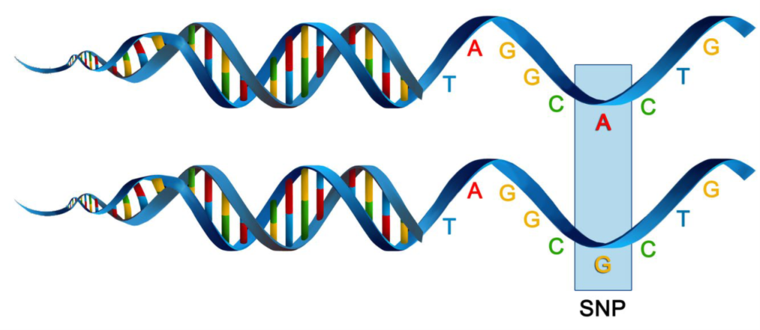
Because it is extremely rare for a mutation to occur twice at the same site in the genome (perhaps with the exception of Eucalypts), the SNP data are considered to be effectively biallelic. Sites with more than two states that occur rarely are typically eliminated in the quality control steps as they are bundled with multiallelic sites arising from multiple copy sequences (e.g. as would arise from gene duplications) removed during preliminary filtering.

The data can be represented as SNP bases (A, T, C or G), with two states for each individual at each locus in a diploid organisms. Alternatively, because the data are biallelic, it is computationally convenient to code the data as 0 for homozyogotes for one allele, 1 for heterozygotes, and 2 for homozygotes of the other allele. The reference allele is arbitrarily taken to be the most common allele, so 0 is the score for homozygous reference, and 2 is the score for homozygous alternate or SNP state. NA indicates that the SNP could not be scored.

SNP data when using dartR are held in a genlight object that is defined in R package adegenet (Jombart, 2008; Jombart and Ahmed, 2011). The locus metadata included in the genlight object are those provided as part of your Diversity Arrays Technology report. These metadata are obtained from the Diversity Arrays Technology csv file when it is read in to the genlight object. The locus metadata are held in an R data.frame that is associated with the SNP data as part of the genlight object.

Here is an example of the data structure of a genlight object

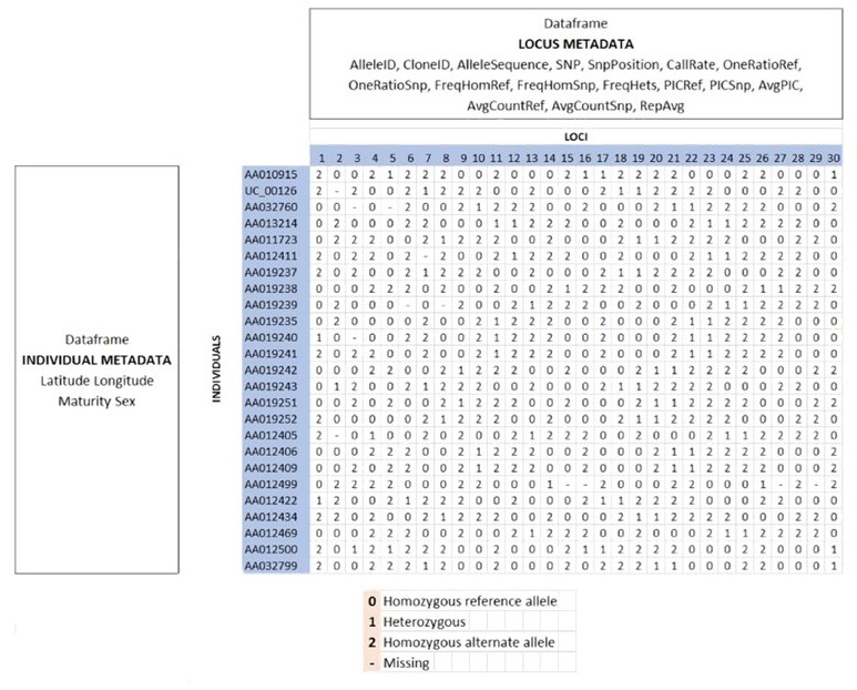
For further details go check out the Data Structure tutorial.

dartR Fundamentals

To help us get our head around data interrogation, subsetting, and basic filtering we are going to work through a worked example using a test dataset.

# dartR comes with a built in test dataset called testset.gl. 
# We first examine the contents of testset.gl
testset.gl

Question time

This is referring to the testset.gl data set you have interrogated above.

How many individuals have been genotyped?

How many SNP loci have been scored?

What is the percentage of missing data?

# Next let us copy the contents of testset.gl to another genlight object called gl.
gl <- testset.gl
# Use adegenet accessors to interrogate the genlight object further
nInd(gl)
nLoc(gl)
nPop(gl)
popNames(gl)
indNames(gl)
locNames(gl)

Now you have a better appreciation of the contents of genlight object gl. pop(gl) is a vector of population names against each individual. Note that it is distinguished from popNames(gl) which just lists the unique names.

# So if you want to tablulate the number of individuals in each population, use
table(pop(gl))

   EmmacBrisWive    EmmacBurdMist    EmmacBurnBara    EmmacClarJack 
              10               10               11                5 
   EmmacClarYate    EmmacCoopAvin   EmmacCoopCully    EmmacCoopEulb 
               5               10               10               10 
  EmmacFitzAllig    EmmacJohnWari    EmmacMaclGeor    EmmacMaryBoru 
              10               10               11                6 
   EmmacMaryPetr     EmmacMDBBowm     EmmacMDBCond     EmmacMDBCudg 
               4               10               10               10 
    EmmacMDBForb     EmmacMDBGwyd     EmmacMDBMaci EmmacMDBMurrMung 
              11                9               10               10 
    EmmacMDBSanf    EmmacNormJack    EmmacNormLeic    EmmacNormSalt 
              10                6                1                1 
   EmmacRichCasi        EmmacRoss    EmmacRussEube     EmmacTweeUki 
              10               10               10               10 
   EmsubRopeMata    EmvicVictJasp 
               5                5 

We have learned that typing the name of the genlight object gives its attributes. How do we examine the genotypes in a genlight object. This is done by converting it to a matrix.

as.matrix(gl)[1:7,1:4]

         100049687-12-C/T 100049698-16-G/A 100049728-23-A/G 100049805-56-T/A
AA010915                2               NA                0                0
UC_00126                2               NA                0                0
AA032760               NA               NA                0                0
AA013214                2               NA                0                0
AA011723                2               NA                0                0
AA012411                2               NA                0                0
AA019237                2               NA                0                0

What do you see? Is it what you expected for the coding of the SNP scores?

Reporting

Lets start over with a focus on reporting.

# Copy the original testset.gl
gl <- testset.gl
# Set the global verbosity to 3 – this will result in some detailed comments 
#  as you run each # script
gl.set.verbosity(3)
# Now lets use a report function to report the call rate for genlight object gl
gl.report.callrate(gl)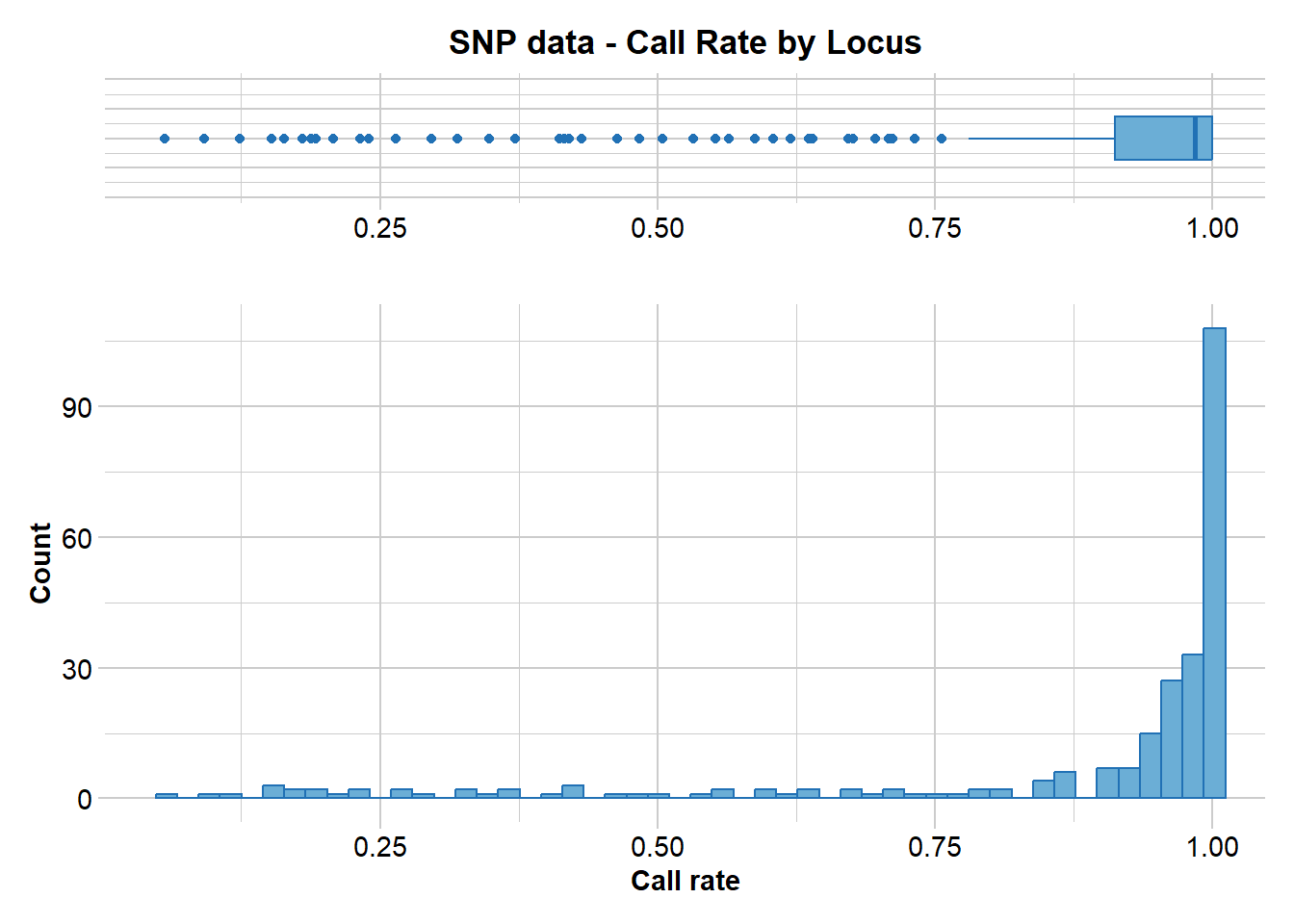

Tip

Note that the call rate is reported against locus. This is the default. Both a tabulated result and a graph is produced. You can use both to determine a suitable threshold for filtering on callrate.

What threshold do you think might be appropriate?

Now let’s report the call rate for genlight object gl by individual.

gl.report.callrate(gl,method="ind")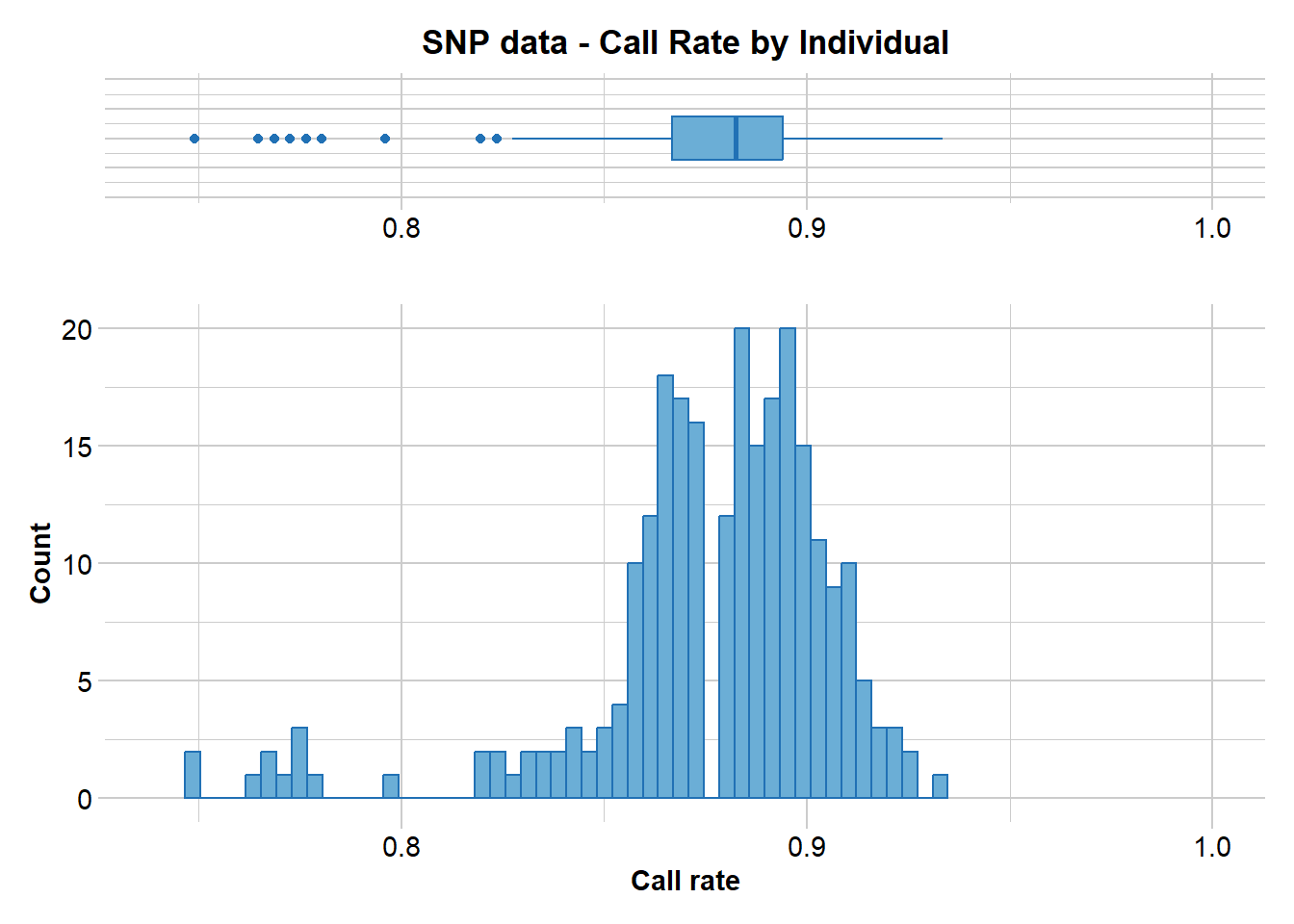

Can you see the difference. Again, both a tabulated result and a graph is produced. You can use both to determine a suitable threshold for filtering on callrate. What threshold do you think might be appropriate?

What about reproducibility?

gl.report.reproducibility(gl)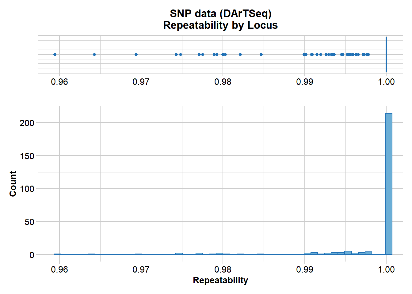

Tip

Recall that DArT runs a series of technical replicates as part of its routine workflow. This enables an assessment of the quality of data associated with each locus. What threshold do you think might be appropriate for a filter of reproducability?

Filtering

Now let’s try some filtering. Return to call rate.

# First look at a report to decide a threshold
gl.report.callrate(gl,method="ind")

Starting gl.report.callrate 
  Processing genlight object with SNP data

  Reporting Call Rate by Individual
  No. of loci = 255 
  No. of individuals = 250 
    Minimum      :  0.7490196 
    1st quartile :  0.8666667 
    Median       :  0.8823529 
    Mean         :  0.8765804 
    3r quartile  :  0.8941176 
    Maximum      :  0.9333333 
    Missing Rate Overall:  0.1234 

Listing 30 populations and their average CallRates
  Monitor again after filtering
         Population CallRate  N
1     EmmacBrisWive   0.8839 10
2     EmmacBurdMist   0.8808 10
3     EmmacBurnBara   0.8859 11
4     EmmacClarJack   0.8596  5
5     EmmacClarYate   0.8769  5
6     EmmacCoopAvin   0.7682 10
7    EmmacCoopCully   0.9122 10
8     EmmacCoopEulb   0.8702 10
9    EmmacFitzAllig   0.8973 10
10    EmmacJohnWari   0.8929 10
11    EmmacMaclGeor   0.8806 11
12    EmmacMaryBoru   0.8843  6
13    EmmacMaryPetr   0.8892  4
14     EmmacMDBBowm   0.8824 10
15     EmmacMDBCond   0.8855 10
16     EmmacMDBCudg   0.8878 10
17     EmmacMDBForb   0.8766 11
18     EmmacMDBGwyd   0.9050  9
19     EmmacMDBMaci   0.8773 10
20 EmmacMDBMurrMung   0.8890 10
21     EmmacMDBSanf   0.8914 10
22    EmmacNormJack   0.8725  6
23    EmmacNormLeic   0.8863  1
24    EmmacNormSalt   0.8706  1
25    EmmacRichCasi   0.8757 10
26        EmmacRoss   0.8706 10
27    EmmacRussEube   0.8612 10
28     EmmacTweeUki   0.8773 10
29    EmsubRopeMata   0.8345  5
30    EmvicVictJasp   0.8361  5

Listing 20 individuals with the lowest CallRates
  Use this list to see which individuals will be lost on filtering by individual
  Set ind.to.list parameter to see more individuals
   Individual    Population  CallRate
1    AA063722 EmmacCoopAvin 0.7490196
2    AA063726 EmmacCoopAvin 0.7490196
3    AA063732 EmmacCoopAvin 0.7647059
4    AA063720 EmmacCoopAvin 0.7686275
5    AA063712 EmmacCoopAvin 0.7686275
6    AA063708 EmmacCoopAvin 0.7725490
7    AA063718 EmmacCoopAvin 0.7764706
8    AA063710 EmmacCoopAvin 0.7764706
9    AA063714 EmmacCoopAvin 0.7764706
10   AA063716 EmmacCoopAvin 0.7803922
11   AA032760  EmmacMDBMaci 0.7960784
12   UC_00210 EmsubRopeMata 0.8196078
13   UC_00259 EmvicVictJasp 0.8196078
14   AA018494 EmmacRichCasi 0.8235294
15   UC_00206 EmsubRopeMata 0.8235294
16   AA019164 EmmacRussEube 0.8274510
17   UC_00209 EmsubRopeMata 0.8313725
18   UC_00254 EmvicVictJasp 0.8313725
19   AA019159 EmmacRussEube 0.8352941
20  UC_00126c EmvicVictJasp 0.8352941

)

Completed: gl.report.callrate 

# Then filter using that threshold
gl <- gl.filter.callrate(gl, method="ind", threshold=0.80)

Starting gl.filter.callrate 
  Processing genlight object with SNP data
  Warning: Data may include monomorphic loci in call rate 
                    calculations for filtering
  Recalculating Call Rate
  Removing individuals based on Call Rate, threshold = 0.8 
  Individuals deleted (CallRate <=  0.8 ):
AA032760[EmmacMDBMaci], AA063718[EmmacCoopAvin], AA063720[EmmacCoopAvin], AA063722[EmmacCoopAvin], AA063726[EmmacCoopAvin], AA063732[EmmacCoopAvin], AA063708[EmmacCoopAvin], AA063710[EmmacCoopAvin], AA063712[EmmacCoopAvin], AA063714[EmmacCoopAvin], AA063716[EmmacCoopAvin],
  Summary of filtered dataset
    Call Rate for individuals > 0.8 
    Original No. of loci : 255 
    Original No. of individuals: 250 
    No. of loci retained: 255 
    No. of individuals retained: 239 
    No. of populations:  29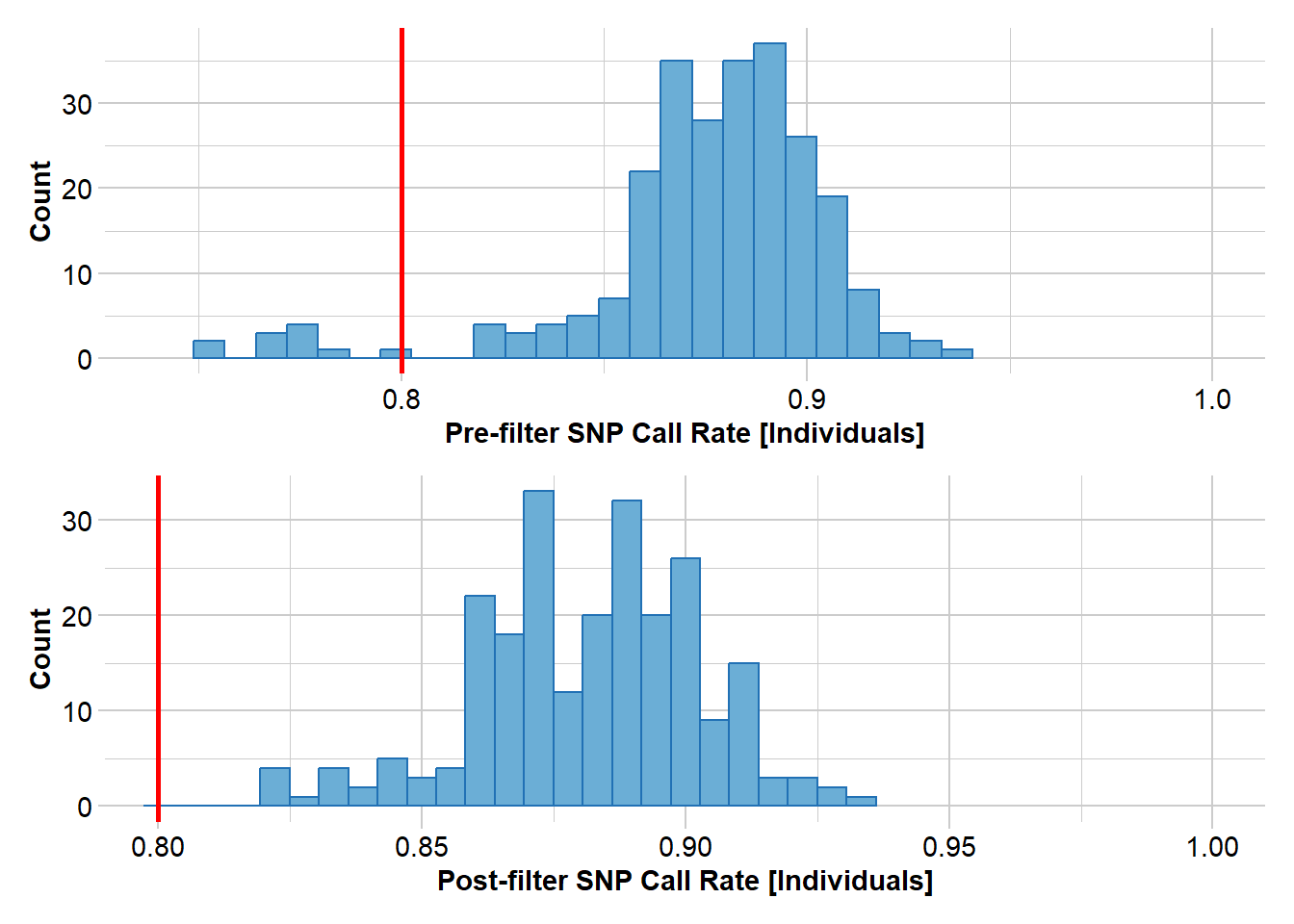 

  Note: Locus metrics not recalculated
  Note: Resultant monomorphic loci not deleted
Completed: gl.filter.callrate 

# Use a smear plot for a visual assessment of the effectiveness of filtering
gl <- testset.gl
smear_pre <- gl.smearplot(gl)

  Processing genlight object with SNP data
Starting gl.smearplot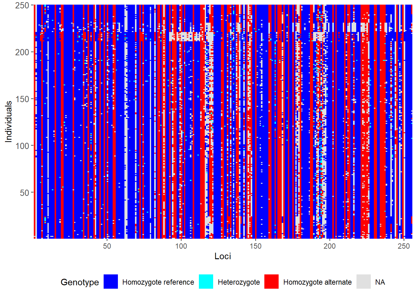 

Completed: gl.smearplot 

Tip

Note the whitespace, which indicates missing data.

# Filter on callrate by locus, then on individual
gl <- gl.filter.callrate(gl,verbose=0)
gl <- gl.filter.callrate(gl, method= "ind", threshold=0.80, verbose=0)

# Examine the smearplot again
smear_post <- gl.smearplot(gl)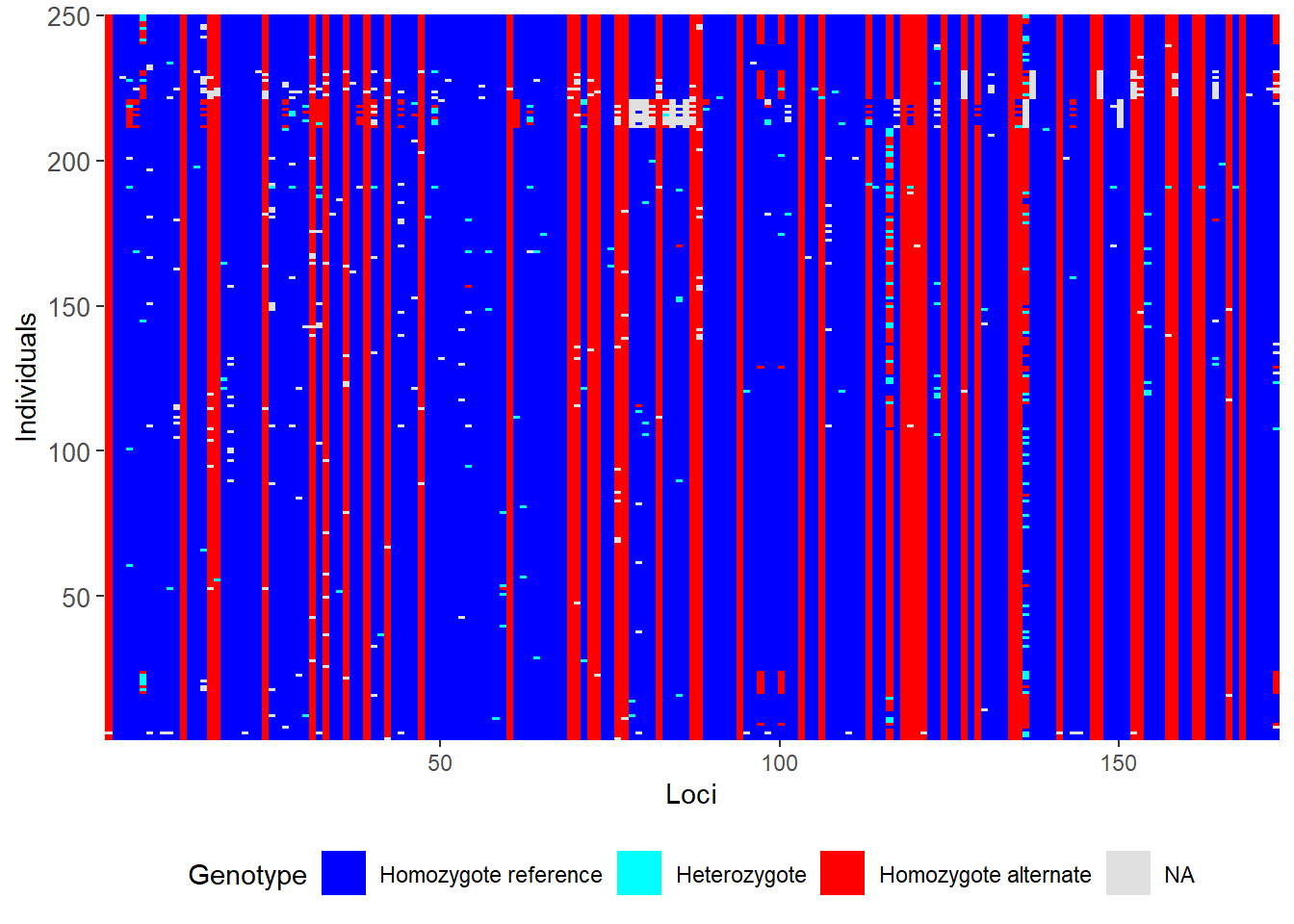

What has happened. What do you conclude?

Filtering out sex-linked markers

For this exercise we will use the data of the Leadbeater’s possum (LBP). This data is included in the package dartR.sexlinked

The Leadbeater’s possum :)

Load data

LBP                   # Explore the dataset
LBP@n.loc             # Number of SNPs
length(LBP@ind.names) # Number of individuals

Question time

How many SNPs and individuals does the LBP genlight object have?

Run gl.report.sexlinked

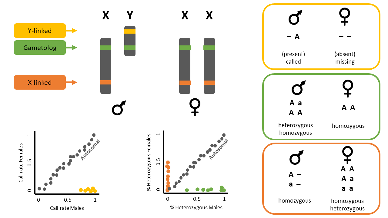
This function identifies sex-linked and autosomal loci present in a SNP dataset (i.e., genlight object) using individuals with known sex. It identifies five types of loci: w-linked or y-linked, sex-biased, z-linked or x-linked, gametologous and autosomal.

Tip

The genlight object must contain in gl@other$ind.metrics a column named id, and a column named sex in which individuals with known-sex are assigned M for male, or F for female. The function ignores individuals that are assigned anything else or nothing at all (unknown-sex).

Check

Check that ind.metrics has the necessary columns:

head(LBP@other$ind.metrics)

	id	sex	pop	Year.collected	service	plate_location
Y2	Y2	F	Yellingbo	1997	DLpos17-2786	1-A1
Y16	Y16	M	Yellingbo	2001	DLpos17-2786	1-A10
Y17	Y17	F	Yellingbo	1997	DLpos17-2786	1-A11
Y18	Y18	F	Yellingbo	1999	DLpos17-2786	1-A12
Y3	Y3	F	Yellingbo	1997	DLpos17-2786	1-A2
Y4	Y4	M	Yellingbo	1997	DLpos17-2786	1-A3

Check

Check the manual of function gl.report.sexlinked to investigate its other requirements:

help(gl.report.sexlinked)

Run the function to identify sex-linked loci in the LBP genlight object:

out <- gl.report.sexlinked(LBP, system = "xy")

Starting gl.report.sexlinked 
  Processing genlight object with SNP data

Detected 162 females and 211 males.

Starting phase 1. May take a while...

Building call rate plot.

Done building call rate plot.

Starting phase 2. May take a while...

Building heterozygosity plot.

Done building heterozygosity plot.

**FINISHED** Total of analyzed loci: 1000.
Found 77 sex-linked loci:
   1 Y-linked loci (yellow)
   9 sex-biased loci (blue)
   66 X-linked loci (orange)
   1 gametologs (green).
And 923 autosomal loci (grey).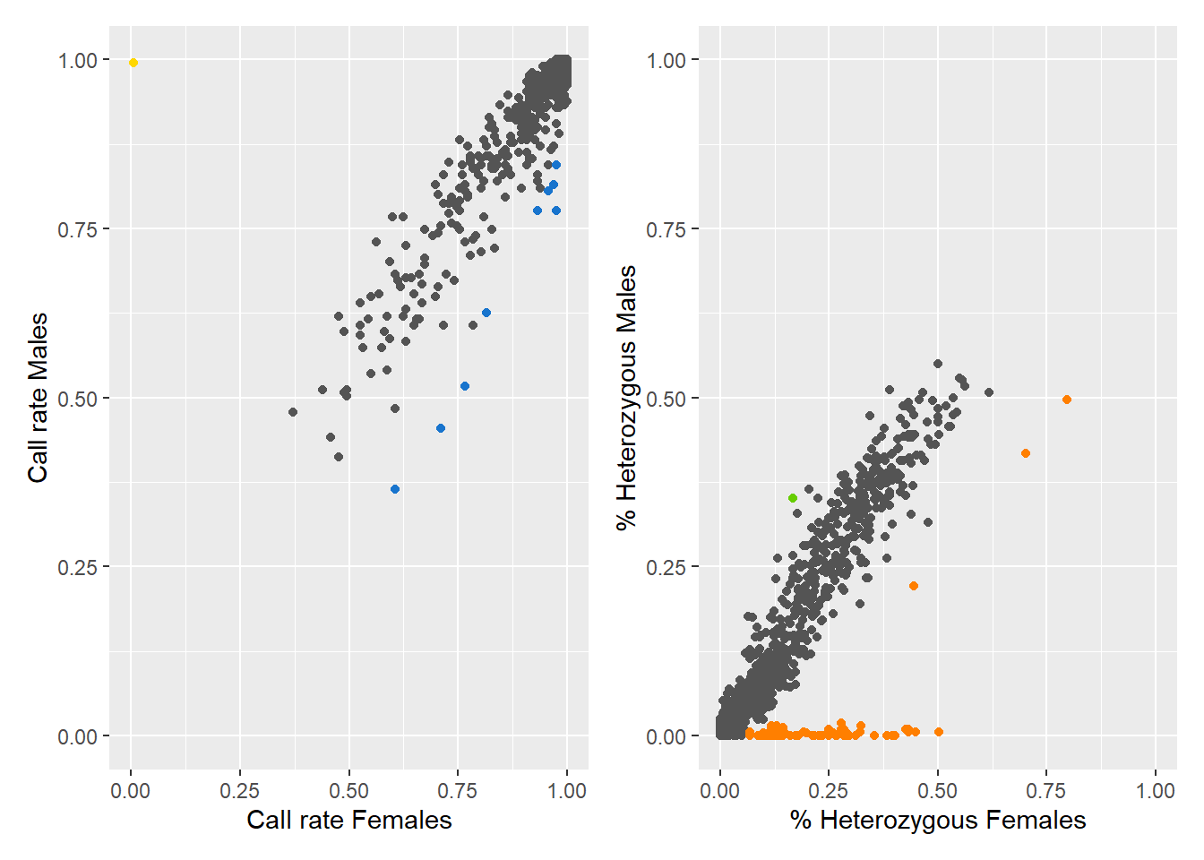

Completed: gl.report.sexlinked 

Question time

Question: Why are we using “xy”?

Question: How many males and females does the dataset contain?

Question: How many sex-linked loci were found?

The output consists of two plots, plus a table. Examine the plots.

Question: What do the colours mean in the plots? Look at the figure below for a hint.

Sex-linked loci in XY sex determination systems

Output dataframe

Now check the output table

out

	index	count.F.miss	count.M.miss	count.F.scored	count.M.scored	ratio	p.value	p.adjusted	scoringRate.F	scoringRate.M	y.linked	sex.biased	count.F.het	count.M.het	count.F.hom	count.M.hom	stat	stat.p.value	stat.p.adjusted	heterozygosity.F	heterozygosity.M	x.linked	gametolog
28681424-34-G/T	1	0	1	162	210	1.2953770	1.0000000	1	1.0000000	0.9952607	FALSE	FALSE	1	0	161	210	1.303397	1.0000000	1.0000000	0.0061728	0.0000000	FALSE	FALSE
28678947-56-C/T	2	12	8	150	203	2.0261283	0.1638428	1	0.9259259	0.9620853	FALSE	FALSE	9	7	141	196	1.784196	0.3044519	0.9598961	0.0600000	0.0344828	FALSE	FALSE
28680567-32-T/G	3	12	12	150	199	1.3256351	0.5289429	1	0.9259259	0.9431280	FALSE	FALSE	9	11	141	188	1.090635	1.0000000	1.0000000	0.0600000	0.0552764	FALSE	FALSE
28688313-7-C/G	4	0	0	162	211	1.3015303	1.0000000	1	1.0000000	1.0000000	FALSE	FALSE	6	0	156	211	8.076192	0.0459068	0.3917911	0.0370370	0.0000000	FALSE	FALSE
28681679-51-C/T	5	22	30	140	181	0.9482168	0.8814171	1	0.8641975	0.8578199	FALSE	FALSE	1	1	139	180	1.293900	1.0000000	1.0000000	0.0071429	0.0055249	FALSE	FALSE
28681994-14-G/A	6	0	1	162	210	1.2953770	1.0000000	1	1.0000000	0.9952607	FALSE	FALSE	18	19	144	191	1.255791	0.6007790	1.0000000	0.1111111	0.0904762	FALSE	FALSE
28687273-35-G/A	7	2	2	160	209	1.3052926	1.0000000	1	0.9876543	0.9905213	FALSE	FALSE	64	81	96	128	1.053325	0.8302485	1.0000000	0.4000000	0.3875598	FALSE	FALSE

only showing the first 7 rows

Run gl.drop.sexlinked

Remove the sex-linked loci from the LBP genlight object:

new.gl <- gl.drop.sexlinked(LBP, system = "xy")

new.gl
new.gl@n.loc

Question time

How many SNPs are there left after removing sex-linked loci?

More filtering

Knock yourself out trying all the different report and filtering functions

Tip

Remember to use them as pairs – report function to decide a threshold, filter function to apply the threshold (where appropriate)

Below are two tables with a number of report and filter functions you can try.

Report functions

Report functions	description
gl.report.callrate	summarises CallRate values
gl.report.reproducibility	summarises repAvg (SNP) or reproducibility (SilicoDArT) values.
gl. report.monomorphs	provides a count of polymorphic and monomorphic loci
gl.report.secondaries	provides a count of loci that are secondaries, that is, loci that reside on the one sequence tag.
gl.report.rdepth	reports the estimate of average read depth for each locus
gl.report.hamming	reports on Hamming distances between sequence tags
gl.report.overshoot	reports loci for which the SNP has been trimmed along with the adaptor sequence
gl.report.taglength	reports a frequency tabulation of sequence tag lengths
gl.report.sexlinked	reports the number and type of loci likely to be in sex chromosomes

Filtering functions

Filter functions	description
gl.filter.callrate	filter out loci or individuals for which the call rate (rate of non-missing values) is less than a specified threshold, say threshold = 0.95
gl.filter.reproducibility	filter out loci for which the reproducibility (strictly repeatability) is less than a specified threshold, say threshold = 0.99
gl. filter.monomorphs	provides a count of polymorphic and monomorphic loci
gl.filter.allna	filter out loci that are all missing values (NA)
gl.filter.secondaries	filter out SNPs that share a sequence tag, except one retained at random [or the best based on reproducibility (RepAvg) and information content (AvgPIC)].
gl.filter.rdepth	filter out loci with exceptionally low or high read depth (coverage)
gl.filter.hamming	filter out loci that differ from each other by less than a specified number of base pairs
gl.filter.overshoot	filter out loci where the SNP location lies outside the trimmed sequence tag
gl.filter.taglength	filter out loci for which the tag length is less that a threshold
gl.filter.sexlinked	filter out loci that are likely to be in sex chromosomes

Exercise

How about trying it with a different dataset?

# how to load a genlight object
gl <- gl.read.dart(filename="./data/sample_data_2row.csv", 
                   ind.metafile="./data/sample_metadata.csv")

You can even try it with your own data.

Further Study

For more tuturials see the dartR Tutorials section.

Check out the other functions contained in package dartR.sexlinked. What do they do?

Keep your eyes peeled for Session 8!

Readings

Gruber et al. (2018)

Mijangos et al. (2022)

Jombart and Ahmed (2011)

Robledo-Ruiz et al. (2023)

Gruber, Bernd, Peter J. Unmack, Oliver F. Berry, and Arthur Georges. 2018. “DARTR : An R Package to Facilitate Analysis of SNP Data Generated from Reduced Representation Genome Sequencing.” Molecular Ecology Resources 18 (3): 691–99. https://doi.org/10.1111/1755-0998.12745.

Jombart, T., and I. Ahmed. 2011. “Adegenet 1.3-1: New Tools for the Analysis of Genome-Wide SNP Data.” Bioinformatics. https://doi.org/10.1093/bioinformatics/btr521.

Mijangos, Jose Luis, Bernd Gruber, Oliver Berry, Carlo Pacioni, and Arthur Georges. 2022. “dartR V2: An Accessible Genetic Analysis Platform for Conservation, Ecology and Agriculture.” Methods in Ecology and Evolution 13 (10): 2150–58. https://doi.org/10.1111/2041-210X.13918.

Robledo-Ruiz, Diana A., Lana Austin, J. Nevil Amos, Jesús Castrejón-Figueroa, Daniel K. P. Harley, Michael J. L. Magrath, Paul Sunnucks, and Alexandra Pavlova. 2023. “Easy-to-Use R Functions to Separate Reduced-Representation Genomic Datasets into Sex-Linked and Autosomal Loci, and Conduct Sex Assignment.” Molecular Ecology Resources 0 (n/a). https://doi.org/10.1111/1755-0998.13844.