6 SNP Panel Selection & Simulations for Conservation

Session Presenters

Required packages

library(dartRverse)
library(knitr)

Introduction

How to go from tens of thousands of SNPs across the genome to just 100?

This session will cover the selection of SNP panels for conservation genetics. We will explore how to select SNPs that are informative for population structure, inbreeding, and other conservation-related analyses. The session will include practical exercises using R and the dartRverse packages.

SNP panels can be used to address either specific questions or to span multiple conservation genetic applications

Population assignment
Parentage or relatedness
Individual ID
Hybridisation
Additional metrics
- Sex-linked SNPs
- Candidate adaptive markers
- Diagnostic SNPs for population ID
- Phenotypic markers

There are a few requirements, like an existing genome wide SNP dataset and good geographical coverage.

Selecting panels

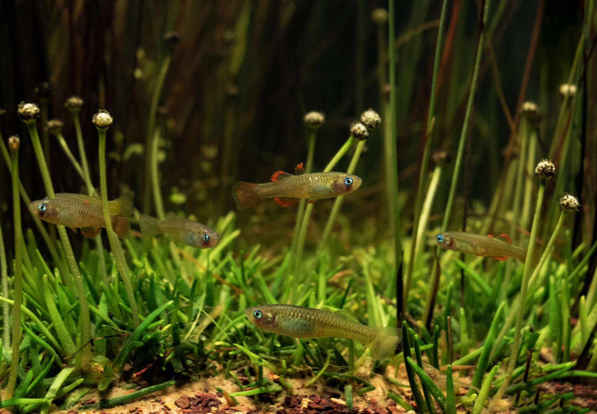
To select panels we will use an example dataset of a fish species as introduced by the slides. The idea is to select a SNP panel that helps to monitor the species. Key aspects to consider a panel is to think about the following:

What is the purpose of the panel? (estimates of Ne, Ho, Fst or all of the above)
How many SNPs can you afford to sequence?

Once you decided on those aspects, you can use the dartRverse package to select a panel of SNPs. The package provides functions to - 1. filter SNPs based on various criteria, mainly for quality - 2. filter SNPs in accordance lab consideration (mainly can we get reliable sequences from the SNPs) - 3. select of the remaining SNPs an informative subsample for the purpose of the panel

Load data

The first two decisions are that we would like to create a SNP panel that is informative for population structure (Fst) and we have resources to develop a panel of 50 SNPs.

Lets load our example data

rfbe <- readRDS("./data/rfbe.rds")
gl.report.basics(rfbe)

Starting gl.report.basics 

SUMMARY STATISTICS

Datatype: SNP 
Loci: 9849 
Individuals: 383 
Populations: 16 

Average Read Depth: 28.70085
Values: 3772167 
           0    1    2   NA
percent 65.5 22.0 11.2  1.3

Monomorphic Loci: 2 
Loci all NA: 0 
Individuals all NA: 0 

Sample Sizes:

    BHA_A2       E504       E508       E509       E518       NW30       NW70 
        19         19         20         20         20         20         20 
      NW72       NW80 PJTub1.2.3   PJTub4.5     PJTub6       SE60       SW10 
        10         10         64         51         33         20         19 
      SW20       SW60 
        18         20 

Loci all NA across individuals by Population
 BHA_A2 E504 E508 E509 E518 NW30 NW70 NW72 NW80 PJTub1.2.3 PJTub4.5 PJTub6 SE60
      0    0    0    0    0    0    0    0    0          0        0      0    0
 SW10 SW20 SW60
    0    0    0

Individuals all NA across loci by Population
 BHA_A2 E504 E508 E509 E518 NW30 NW70 NW72 NW80 PJTub1.2.3 PJTub4.5 PJTub6 SE60
      0    0    0    0    0    0    0    0    0          0        0      0    0
 SW10 SW20 SW60
    0    0    0

Completed: gl.report.basics

Filtering for quality

So we have 9849 SNPs (they are prefiltered for quality already). You can check the looking at callrate, rdepth). So we already have high quality SNPs, with a low missing value rate across loci.

our main aim is to find a panel of 50 SNPs that are informative for population structure (Fst).

To be able to calculate Fst reliably we decided to have a threshold of more than 10 individuals per population so we filter the SNPs for a minimum of 11 individuals per population.

tt <- table(pop(rfbe))
pop20 <- names(tt)[tt>10]

rfbe20 <- gl.keep.pop(rfbe, pop.list=pop20)

Starting gl.keep.pop 
  Processing genlight object with SNP data
  Checking for presence of nominated populations
  Retaining only populations BHA_A2, E504, E508, E509, E518, NW30, NW70, PJTub1.2.3, PJTub4.5, PJTub6, SE60, SW10, SW20, SW60 
  Warning: Resultant dataset may contain monomorphic loci
  Locus metrics not recalculated
Completed: gl.keep.pop

kable(table(pop(rfbe20)))

Var1	Freq
BHA_A2	19
E504	19
E508	20
E509	20
E518	20
NW30	20
NW70	20
PJTub1.2.3	64
PJTub4.5	51
PJTub6	33
SE60	20
SW10	19
SW20	18
SW60	20

Because we have filtered the data by individual we want to make sure we have not created missing data in any of the populations and we want to filter also finally for minor allele frequency (MAF) using the count option as we want to make sure we have high quality SNPs which are not spurious in terms of aonly occuring in very low frequency.

You can use the report function before filtering to test their effect.

rfbe20_1 <- gl.filter.allna(rfbe20, by.pop = T)

Starting gl.filter.allna 
  Identifying and removing loci that are all missing (NA) 
                    in any one population
  Deleting loci that are all missing (NA) in any one population
  Warning: no loci listed to delete! Genlight object returned unchanged
Completed: gl.filter.allna

rfbe20_2 <- gl.filter.callrate(rfbe20_1, threshold=0.99)

Starting gl.filter.callrate 
  Processing genlight object with SNP data
  Warning: Data may include monomorphic loci in call rate 
                    calculations for filtering
  Recalculating Call Rate
  Removing loci based on Call Rate, threshold = 0.99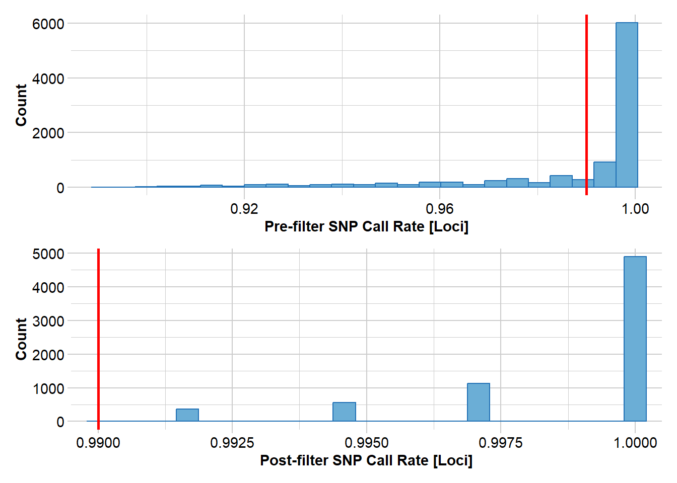

Completed: gl.filter.callrate

rfbe20_3 <- gl.filter.maf(rfbe20_2, threshold = 5, by.pop = FALSE)

Starting gl.filter.maf 
  Processing genlight object with SNP data
  Warning: genlight object contains monomorphic loci
  Removing loci with MAF < 0.0068870523415978 over all the dataset
                and recalculating FreqHoms and FreqHets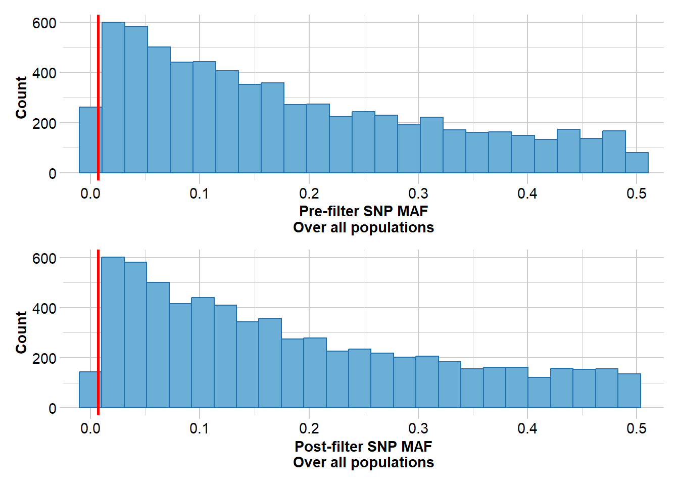

Completed: gl.filter.maf

nLoc(rfbe20_3)

[1] 6815

This should result in high quality SNPs.

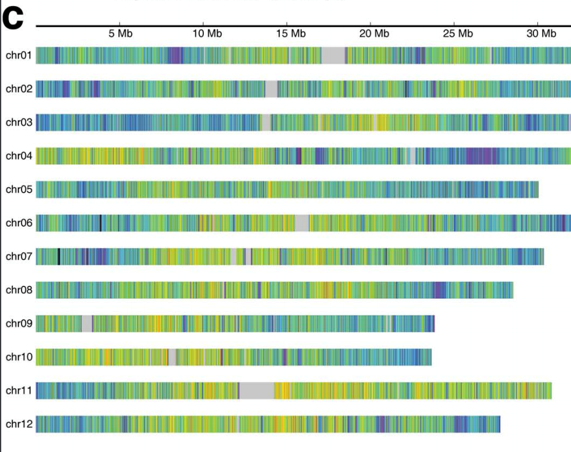
If you have a reference genome you would like to filter for SNPs that are 100% aligned and of a certain length. For example you want to make sure the sequences you have are at least of a certain length.

Filter SNPs with sequences that are less than 30 characters long

index <- nchar(as.character(rfbe20_3@other$loc.metrics$TrimmedSequence))>29
rfbe20_4 <- rfbe20_3[, index]

As we have a reference genome we include another step, manly to filter for SNPs that are aligned very well to the reference genome. This is important and can help if your SNP is towards the beginning of your sequence but you want to design primers that have the SNP more towards the middle of a sequence.

blast to find SNPs

#takes a while to run, hence load the pre run data set
#rfbe20_5 <- gl.blast(rfbe20_4,ref_genome="d:/bernd/r/Elise_pansnp/final.genome.scf.fasta", 
#                     task = "blastn", number_of_threads = 10 )
#saveRDS(rfbe20_5, "d:/bernd/r/Elise_pansnp/rfbe20_5_blast.rds")

rfbe20_5 <- readRDS("./data/rfbe20_5_blast.rds")

We can now filter the SNPs based on the blast results.

#bitscore >=100
index <- rfbe20_5@other$loc.metrics$bitscore >= 100
index <- ifelse(is.na(index), FALSE, index)
rfbe20_6 <- rfbe20_5[,index]

Depending on your lab requirements you might want to filter for SNPs that are not too close to close to the beginning of the sequence. As we have a reference genome, that allows us to extend sequences, we do not do that here. In case you are interested we are currently have a semi-developed script that allows to do this, but it is not yet part of the package.

Selecting informative SNPs

We can now select a subsample of SNPs using several different methods. Depending on the aim of your panel you might want to select SNPs that are informative for population structure (Fst) or inbreeding (Ho). It turns out that the dapc method is a good method to select SNPs that are informative for population structure. The code below uses this method to select 50 SNPs.

run `gl.select.panel`

#takes a while to run
panel <- gl.select.panel(rfbe20_6, method="dapc", nl = 50)

Starting gl.select.panel 
  Processing genlight object with SNP data

Found more than one class "dist" in cache; using the first, from namespace 'BiocGenerics'

Also defined by 'spam'

Found more than one class "dist" in cache; using the first, from namespace 'BiocGenerics'

Also defined by 'spam'

Starting gl.keep.loc 
  Processing genlight object with SNP data
  List of loci to keep has been specified
  Deleting all but the specified loci
Completed: gl.keep.loc 
Completed: gl.select.panel

nLoc(panel)

[1] 66

run `gl.check.panel`

outdapc <- gl.check.panel(panel, rfbe20_6, parameter = "Fst")

`geom_smooth()` using formula = 'y ~ x'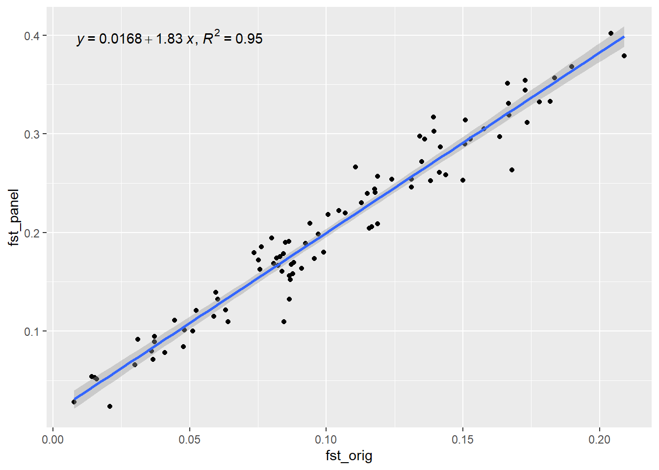

As we can see Fst values between populations is nicely reconstructed by selecting only 50 SNPs based on the dapc method. We can compare it to a random selection:

panel_random <- gl.select.panel(rfbe20_6, method="random", nl = 50)

Starting gl.select.panel 
  Processing genlight object with SNP data
Starting gl.keep.loc 
  Processing genlight object with SNP data
  List of loci to keep has been specified
  Deleting all but the specified loci
Completed: gl.keep.loc 
Completed: gl.select.panel

outrandom <- gl.check.panel(panel_random, rfbe20_6, parameter = "Fst")

`geom_smooth()` using formula = 'y ~ x'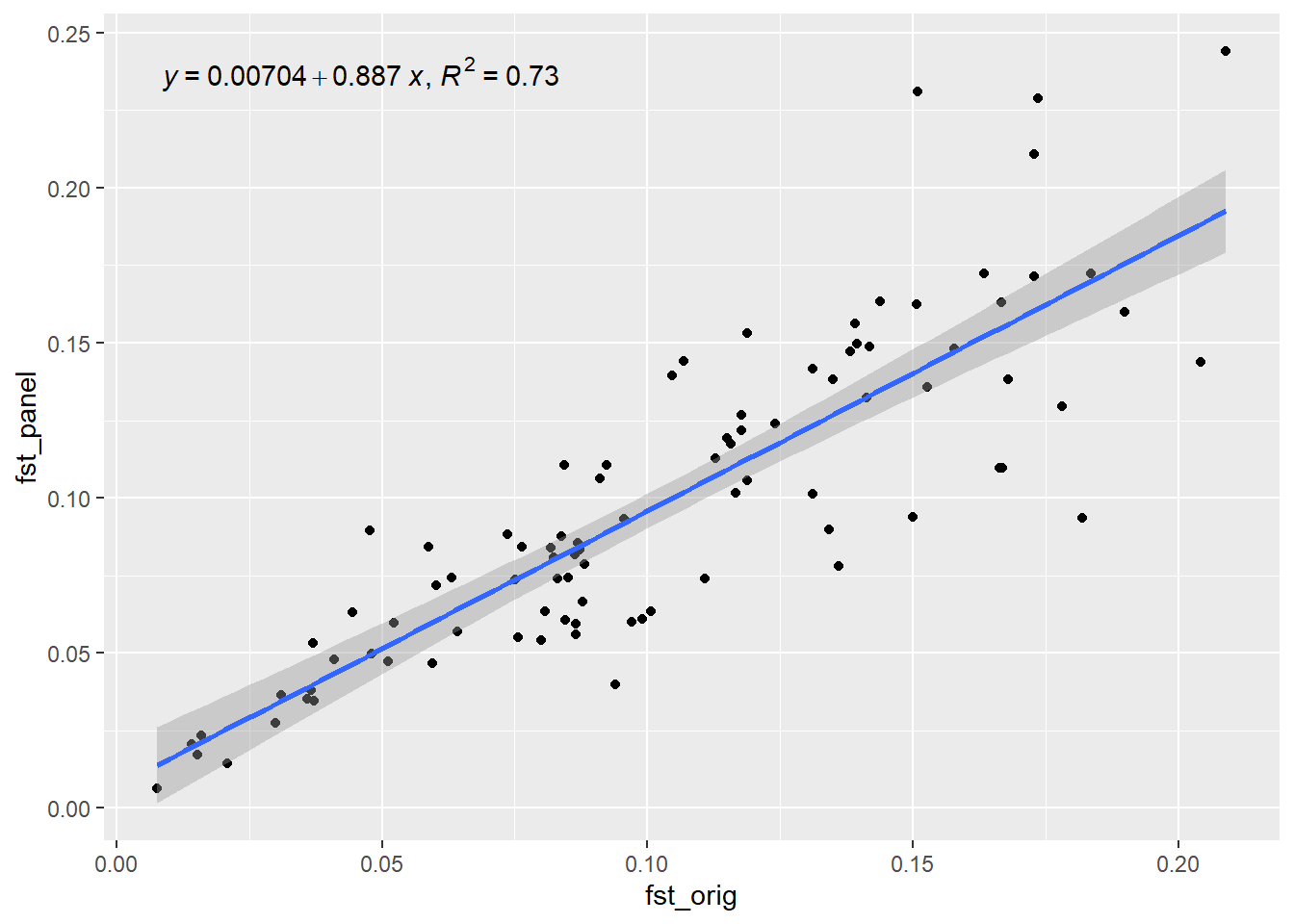

Not as good so it pays off.

Further Study

Exercise

Now it is time for you to select a SNP panel.

You can try different methods and compare them. E.g How good is a random panel, or one based on PIC values.

Required packages

Introduction

Selecting panels

Load data

Filtering for quality

Filter SNPs with sequences that are less than 30 characters long

blast to find SNPs

Selecting informative SNPs

run gl.select.panel

run gl.check.panel

Further Study

Readings

run `gl.select.panel`

run `gl.check.panel`