Reports loci containing secondary SNPs in sequence tags and calculates number of invariant sites

SNP datasets generated by DArT include fragments with more than one SNP (that is, with secondaries). They are recorded separately with the same CloneID (=AlleleID). These multiple SNP loci within a fragment are likely to be linked, and so you may wish to remove secondaries.

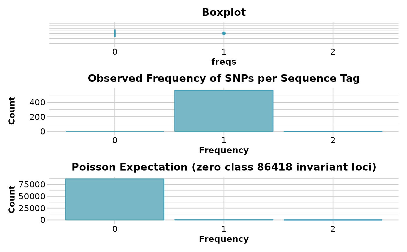
This function reports statistics associated with secondaries, and the consequences of filtering them out, and provides three plots. The first is a boxplot, the second is a barplot of the frequency of secondaries per sequence tag, and the third is the Poisson expectation for those frequencies including an estimate of the zero class (no. of sequence tags with no SNP scored).

gl.report.secondaries(
  x,
  nsim = 1000,
  taglength = 69,
  plot.out = TRUE,
  plot_theme = theme_dartR(),
  plot_colors = two_colors,
  save2tmp = FALSE,
  verbose = NULL
)

Arguments

x

Name of the genlight object containing the SNP data [required].

nsim

The number of simulations to estimate the mean of the Poisson distribution [default 1000].

taglength

Typical length of the sequence tags [default 69].

plot.out

Specify if plot is to be produced [default TRUE].

plot_theme

Theme for the plot. See Details for options [default theme_dartR()].

plot_colors

List of two color names for the borders and fill of the plots [default two_colors].

save2tmp

If TRUE, saves any ggplots and listings to the session temporary directory (tempdir) [default FALSE].

verbose

Verbosity: 0, silent or fatal errors; 1, begin and end; 2, progress log; 3, progress and results summary; 5, full report [default 2, unless specified using gl.set.verbosity].

Value

A data.frame with the list of parameter values

• n.total.tags Number of sequence tags in total

• n.SNPs.secondaries Number of secondary SNP loci that would be removed on filtering

• n.invariant.tags Estimated number of invariant sequence tags

• n.tags.secondaries Number of sequence tags with secondaries

• n.inv.gen Number of invariant sites in sequenced tags

• mean.len.tag Mean length of sequence tags

• n.invariant Total Number of invariant sites (including invariant sequence tags)

• k Lambda: mean of the Poisson distribution of number of SNPs in the sequence tags

Details

The function gl.filter.secondaries will filter out the loci with secondaries retaining only one sequence tag.

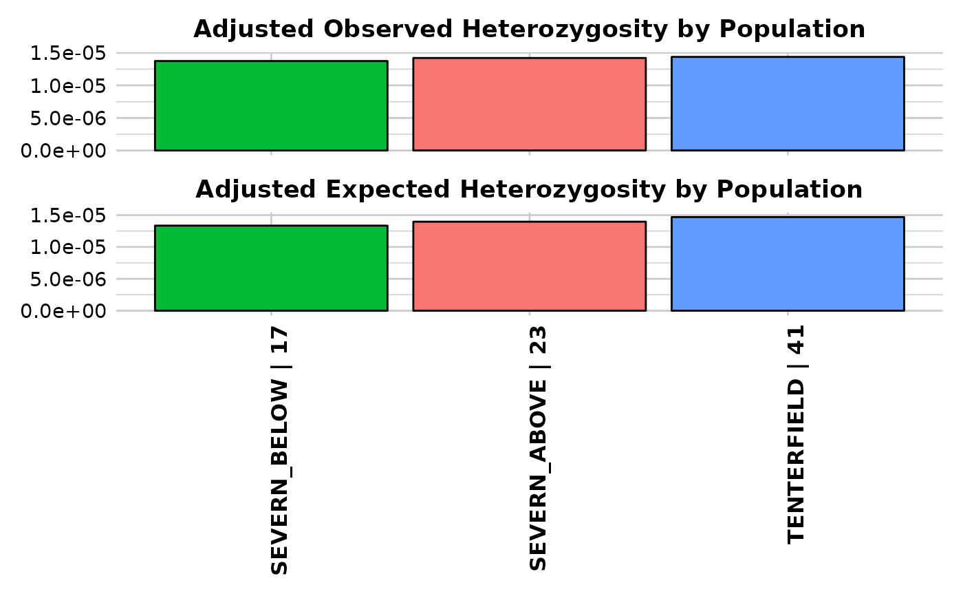
Heterozygosity as estimated by the function gl.report.heterozygosity is in a sense relative, because it is calculated against a background of only those loci that are polymorphic somewhere in the dataset. To allow intercompatibility across studies and species, any measure of heterozygosity needs to accommodate loci that are invariant (autosomal heterozygosity. See Schmidt et al 2021). However, the number of invariant loci are unknown given the SNPs are detected as single point mutational variants and invariant sequences are discarded, and because of the particular additional filtering pre-analysis. Modelling the counts of SNPs per sequence tag as a Poisson distribution in this script allows estimate of the zero class, that is, the number of invariant loci. This is reported, and the veracity of the estimate can be assessed by the correspondence of the observed frequencies against those under Poisson expectation in the associated graphs. The number of invariant loci can then be optionally provided to the function gl.report.heterozygosity via the parameter n.invariants.

In case the calculations for the Poisson expectation of the number of invariant sequence tags fail to converge, try to rerun the analysis with a larger nsim values.

This function now also calculates the number of invariant sites (i.e. nucleotides) of the sequence tags (if TrimmedSequence is present in x$other$loc.metrics) or estimate these by assuming that the average length of the sequence tags is 69 nucleotides. Based on the Poisson expectation of the number of invariant sequence tags, it also estimates the number of invariant sites for these to eventually provide an estimate of the total number of invariant sites.

Note, previous version of dartR would only return an estimate of the number of invariant sequence tags (not sites).

Plots are saved to the session temporary directory (tempdir).

Examples of other themes that can be used can be consulted in:

• https://ggplot2.tidyverse.org/reference/ggtheme.html and

• https://yutannihilation.github.io/allYourFigureAreBelongToUs/ggthemes/

References

Schmidt, T.L., Jasper, M.-E., Weeks, A.R., Hoffmann, A.A., 2021. Unbiased population heterozygosity estimates from genome-wide sequence data. Methods in Ecology and Evolution n/a.

See also

gl.filter.secondaries,gl.report.heterozygosity, utils.n.var.invariant

Other report functions: gl.report.bases(), gl.report.callrate(), gl.report.diversity(), gl.report.hamming(), gl.report.hwe(), gl.report.ld.map(), gl.report.locmetric(), gl.report.maf(), gl.report.monomorphs(), gl.report.overshoot(), gl.report.pa(), gl.report.parent.offspring(), gl.report.rdepth(), gl.report.replicates(), gl.report.reproducibility(), gl.report.sexlinked(), gl.report.taglength()

Author

Custodian: Arthur Georges (Post to https://groups.google.com/d/forum/dartr)

Examples

require("dartR.data")
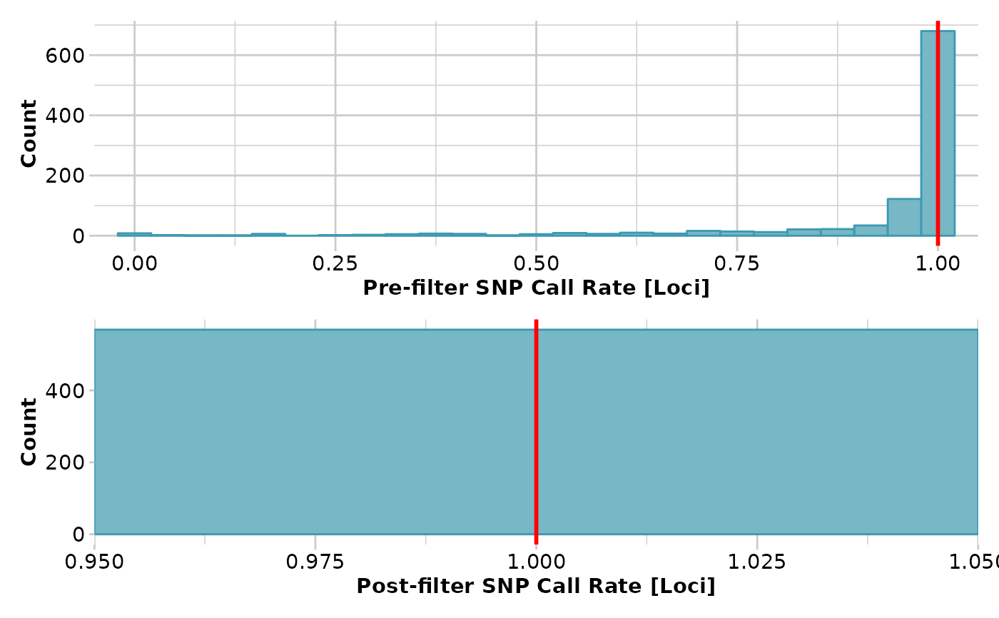
test <- gl.filter.callrate(platypus.gl,threshold = 1)
#> Starting gl.filter.callrate 
#>   Processing genlight object with SNP data
#>   Warning: data include loci that are scored NA across all individuals.
#>   Consider filtering using gl <- gl.filter.allna(gl)
#>   Warning: Data may include monomorphic loci in call rate 
#>                     calculations for filtering
#>   Recalculating Call Rate
#>   Removing loci based on Call Rate, threshold = 1 
#> 

#> Completed: gl.filter.callrate 
#> 
n.inv <- gl.report.secondaries(test)
#> Starting gl.report.secondaries 
#>   Processing genlight object with SNP data
#> Counting ....
#> Estimating parameters (lambda) of the Poisson expectation
#> [1] 1.001761
#> [1] 0.6338817
#> [1] 0.4702981
#> [1] 0.3758445
#> [1] 0.3138425
#> [1] 0.2698401
#> [1] 0.2369148
#> [1] 0.2113129
#> [1] 0.1908146
#> [1] 0.1740201
#> [1] 0.1600012
#> [1] 0.1481175
#> [1] 0.1379126
#> [1] 0.129052
#> [1] 0.1212849
#> [1] 0.1144195
#> [1] 0.1083066
#> [1] 0.1028283
#> [1] 0.09789016
#> [1] 0.09341568
#> [1] 0.08934221
#> [1] 0.08561791
#> [1] 0.08219956
#> [1] 0.0790508
#> [1] 0.07614083
#> [1] 0.07344338
#> [1] 0.07093592
#> [1] 0.06859898
#> [1] 0.06641568
#> [1] 0.06437132
#> [1] 0.06245299
#> [1] 0.06064937
#> [1] 0.05895042
#> [1] 0.05734728
#> [1] 0.05583203
#> [1] 0.05439763
#> [1] 0.05303776
#> [1] 0.05174674
#> [1] 0.05051947
#> [1] 0.04935131
#> [1] 0.0482381
#> [1] 0.04717604
#> [1] 0.04616167
#> [1] 0.04519185
#> [1] 0.0442637
#> [1] 0.04337459
#> [1] 0.0425221
#> [1] 0.04170401
#> [1] 0.04091827
#> [1] 0.04016301
#> [1] 0.03943647
#> [1] 0.03873705
#> [1] 0.03806326
#> [1] 0.03741372
#> [1] 0.03678712
#> [1] 0.03618229
#> [1] 0.03559809
#> [1] 0.0350335
#> [1] 0.03448755
#> [1] 0.03395931
#> [1] 0.03344795
#> [1] 0.03295267
#> [1] 0.03247271
#> [1] 0.03200739
#> [1] 0.03155603
#> [1] 0.03111802
#> [1] 0.03069278
#> [1] 0.03027976
#> [1] 0.02987843
#> [1] 0.0294883
#> [1] 0.02910892
#> [1] 0.02873985
#> [1] 0.02838067
#> [1] 0.02803098
#> [1] 0.02769043
#> [1] 0.02735864
#> [1] 0.0270353
#> [1] 0.02672007
#> [1] 0.02641267
#> [1] 0.0261128
#> [1] 0.02582019
#> [1] 0.02553457
#> [1] 0.02525571
#> [1] 0.02498336
#> [1] 0.0247173
#> [1] 0.02445731
#> [1] 0.02420319
#> [1] 0.02395474
#> [1] 0.02371178
#> [1] 0.02347412
#> [1] 0.02324159
#> [1] 0.02301403
#> [1] 0.02279128
#> [1] 0.02257319
#> [1] 0.02235962
#> [1] 0.02215043
#> [1] 0.02194548
#> [1] 0.02174464
#> [1] 0.0215478
#> [1] 0.02135484
#> [1] 0.02116563
#> [1] 0.02098009
#> [1] 0.02079809
#> [1] 0.02061954
#> [1] 0.02044434
#> [1] 0.0202724
#> [1] 0.02010363
#> [1] 0.01993794
#> [1] 0.01977524
#> [1] 0.01961547
#> [1] 0.01945854
#> [1] 0.01930437
#> [1] 0.01915289
#> [1] 0.01900404
#> [1] 0.01885774
#> [1] 0.01871394
#> [1] 0.01857256
#> [1] 0.01843355
#> [1] 0.01829685
#> [1] 0.0181624
#> [1] 0.01803014
#> [1] 0.01790003
#> [1] 0.01777201
#> [1] 0.01764603
#> [1] 0.01752204
#> [1] 0.01740001
#> [1] 0.01727987
#> [1] 0.01716159
#> [1] 0.01704512
#> [1] 0.01693043
#> [1] 0.01681748
#> [1] 0.01670621
#> [1] 0.0165966
#> [1] 0.01648862
#> [1] 0.01638222
#> [1] 0.01627736
#> [1] 0.01617403
#> [1] 0.01607218
#> [1] 0.01597178
#> [1] 0.0158728
#> [1] 0.01577522
#> [1] 0.015679
#> [1] 0.01558411
#> [1] 0.01549053
#> [1] 0.01539823
#> [1] 0.01530719
#> [1] 0.01521737
#> [1] 0.01512876
#> [1] 0.01504133
#> [1] 0.01495506
#> [1] 0.01486992
#> [1] 0.01478589
#> [1] 0.01470296
#> [1] 0.01462109
#> [1] 0.01454028
#> [1] 0.01446049
#> [1] 0.01438172
#> [1] 0.01430393
#> [1] 0.01422712
#> [1] 0.01415127
#> [1] 0.01407635
#> [1] 0.01400235
#> [1] 0.01392925
#> [1] 0.01385704
#> [1] 0.0137857
#> [1] 0.01371522
#> [1] 0.01364557
#> [1] 0.01357676
#> [1] 0.01350875
#> [1] 0.01344154
#> [1] 0.01337511
#> [1] 0.01330945
#> [1] 0.01324455
#> [1] 0.01318039
#> [1] 0.01311696
#> [1] 0.01305425
#> [1] 0.01299225
#> [1] 0.01293094
#> [1] 0.01287031
#> [1] 0.01281036
#> [1] 0.01275107
#> [1] 0.01269242
#> [1] 0.01263442
#> [1] 0.01257704
#> [1] 0.01252029
#> [1] 0.01246414
#> [1] 0.01240859
#> [1] 0.01235363
#> [1] 0.01229925
#> [1] 0.01224545
#> [1] 0.01219221
#> [1] 0.01213952
#> [1] 0.01208737
#> [1] 0.01203577
#> [1] 0.01198469
#> [1] 0.01193413
#> [1] 0.01188409
#> [1] 0.01183455
#> [1] 0.01178551
#> [1] 0.01173696
#> [1] 0.0116889
#> [1] 0.0116413
#> [1] 0.01159418
#> [1] 0.01154752
#> [1] 0.01150132
#> [1] 0.01145557
#> [1] 0.01141025
#> [1] 0.01136538
#> [1] 0.01132093
#> [1] 0.01127691
#> [1] 0.01123331
#> [1] 0.01119012
#> [1] 0.01114733
#> [1] 0.01110495
#> [1] 0.01106296
#> [1] 0.01102136
#> [1] 0.01098014
#> [1] 0.0109393
#> [1] 0.01089884
#> [1] 0.01085875
#> [1] 0.01081902
#> [1] 0.01077965
#> [1] 0.01074063
#> [1] 0.01070197
#> [1] 0.01066365
#> [1] 0.01062567
#> [1] 0.01058802
#> [1] 0.01055071
#> [1] 0.01051372
#> [1] 0.01047706
#> [1] 0.01044071
#> [1] 0.01040469
#> [1] 0.01036897
#> [1] 0.01033356
#> [1] 0.01029845
#> [1] 0.01026364
#> [1] 0.01022912
#> [1] 0.0101949
#> [1] 0.01016097
#> [1] 0.01012732
#> [1] 0.01009395
#> [1] 0.01006086
#> [1] 0.01002804
#> [1] 0.009995493
#> [1] 0.009963214
#> [1] 0.0099312
#> [1] 0.009899446
#> [1] 0.009867951
#> [1] 0.00983671
#> [1] 0.009805721
#> [1] 0.009774981
#> [1] 0.009744487
#> [1] 0.009714235
#> [1] 0.009684224
#> [1] 0.009654451
#> [1] 0.009624912
#> [1] 0.009595604
#> [1] 0.009566526
#> [1] 0.009537675
#> [1] 0.009509047
#> [1] 0.009480641
#> [1] 0.009452454
#> [1] 0.009424483
#> [1] 0.009396727
#> [1] 0.009369181
#> [1] 0.009341845
#> [1] 0.009314716
#> [1] 0.009287792
#> [1] 0.009261069
#> [1] 0.009234547
#> [1] 0.009208223
#> [1] 0.009182094
#> [1] 0.009156159
#> [1] 0.009130416
#> [1] 0.009104861
#> [1] 0.009079495
#> [1] 0.009054313
#> [1] 0.009029315
#> [1] 0.009004498
#> [1] 0.008979861
#> [1] 0.008955401
#> [1] 0.008931117
#> [1] 0.008907007
#> [1] 0.008883069
#> [1] 0.008859301
#> [1] 0.008835702
#> [1] 0.008812269
#> [1] 0.008789001
#> [1] 0.008765896
#> [1] 0.008742953
#> [1] 0.00872017
#> [1] 0.008697546
#> [1] 0.008675078
#> [1] 0.008652765
#> [1] 0.008630605
#> [1] 0.008608598
#> [1] 0.008586741
#> [1] 0.008565033
#> [1] 0.008543472
#> [1] 0.008522058
#> [1] 0.008500788
#> [1] 0.008479661
#> [1] 0.008458676
#> [1] 0.008437831
#> [1] 0.008417126
#> [1] 0.008396558
#> [1] 0.008376126
#> [1] 0.008355829
#> [1] 0.008335666
#> [1] 0.008315635
#> [1] 0.008295735
#> [1] 0.008275965
#> [1] 0.008256324
#> [1] 0.00823681
#> [1] 0.008217422
#> [1] 0.008198159
#> [1] 0.008179021
#> [1] 0.008160004
#> [1] 0.00814111
#> [1] 0.008122335
#> [1] 0.00810368
#> [1] 0.008085143
#> [1] 0.008066723
#> [1] 0.00804842
#> [1] 0.008030231
#> [1] 0.008012156
#> [1] 0.007994193
#> [1] 0.007976343
#> [1] 0.007958603
#> [1] 0.007940974
#> [1] 0.007923453
#> [1] 0.007906039
#> [1] 0.007888733
#> [1] 0.007871533
#> [1] 0.007854437
#> [1] 0.007837446
#> [1] 0.007820557
#> [1] 0.007803771
#> [1] 0.007787087
#> [1] 0.007770502
#> [1] 0.007754017
#> [1] 0.007737631
#> [1] 0.007721343
#> [1] 0.007705151
#> [1] 0.007689056
#> [1] 0.007673056
#> [1] 0.00765715
#> [1] 0.007641339
#> [1] 0.00762562
#> [1] 0.007609993
#> [1] 0.007594457
#> [1] 0.007579012
#> [1] 0.007563656
#> [1] 0.00754839
#> [1] 0.007533212
#> [1] 0.007518121
#> [1] 0.007503117
#> [1] 0.007488199
#> [1] 0.007473367
#> [1] 0.007458619
#> [1] 0.007443955
#> [1] 0.007429374
#> [1] 0.007414876
#> [1] 0.00740046
#> [1] 0.007386125
#> [1] 0.00737187
#> [1] 0.007357696
#> [1] 0.0073436
#> [1] 0.007329583
#> [1] 0.007315645
#> [1] 0.007301783
#> [1] 0.007287998
#> [1] 0.007274289
#> [1] 0.007260656
#> [1] 0.007247098
#> [1] 0.007233614
#> [1] 0.007220204
#> [1] 0.007206866
#> [1] 0.007193602
#> [1] 0.007180409
#> [1] 0.007167288
#> [1] 0.007154237
#> [1] 0.007141257
#> [1] 0.007128347
#> [1] 0.007115506
#> [1] 0.007102733
#> [1] 0.007090029
#> [1] 0.007077392
#> [1] 0.007064823
#> [1] 0.00705232
#> [1] 0.007039883
#> [1] 0.007027512
#> [1] 0.007015205
#> [1] 0.007002964
#> [1] 0.006990786
#> [1] 0.006978672
#> [1] 0.006966622
#> [1] 0.006954634
#> [1] 0.006942708
#> [1] 0.006930843
#> [1] 0.006919041
#> [1] 0.006907299
#> [1] 0.006895617
#> [1] 0.006883995
#> [1] 0.006872433
#> [1] 0.006860929
#> [1] 0.006849485
#> [1] 0.006838098
#> [1] 0.006826769
#> [1] 0.006815498
#> [1] 0.006804283
#> [1] 0.006793125
#> [1] 0.006782024
#> [1] 0.006770977
#> [1] 0.006759986
#> [1] 0.00674905
#> [1] 0.006738169
#> [1] 0.006727341
#> [1] 0.006716568
#> [1] 0.006705847
#> [1] 0.00669518
#> [1] 0.006684565
#> [1] 0.006674002
#> [1] 0.006663491
#> [1] 0.006653032
#> [1] 0.006642624
#> [1] 0.006632266
#> [1] 0.006621959
#> [1] 0.006611702
#> [1] 0.006601495
#> [1] 0.006591337
#> [1] 0.006581228
#> [1] 0.006571168
#> [1] 0.006561156
#>   Converged on Lambda of 0.00655119223854876 
#> 
#> 

#>   Total number of SNP loci scored: 569 
#>    Number of sequence tags in total: 568 
#>    Estimated number of invariant sequence tags: 86418 
#>    Number of sequence tags with secondaries: 1 
#>    Number of secondary SNP loci that would be removed on 
#>             filtering: 1 
#>    Number of SNP loci that would be retained on filtering: 568 
#>    Number of invariant sites in sequenced tags: 37537 
#>    Mean length of sequence tags: 67.08803 
#>    Total Number of invariant sites (including invariant sequence 
#>             tags): 5835150 
#> Completed: gl.report.secondaries 
#> 
gl.report.heterozygosity(test, n.invariant = n.inv[7, 2])
#> Starting gl.report.heterozygosity 
#>   Processing genlight object with SNP data
#>   Calculating Observed Heterozygosities, averaged across
#>                     loci, for each population
#>   Calculating Expected Heterozygosities
#> 
#> 

#>                       pop n.Ind n.Loc    n.Loc.adj polyLoc monoLoc all_NALoc
#> SEVERN_ABOVE SEVERN_ABOVE    23   569 9.750298e-05     304     265         0
#> SEVERN_BELOW SEVERN_BELOW    17   569 9.750298e-05     279     290         0
#> TENTERFIELD   TENTERFIELD    41   569 9.750298e-05     349     220         0
#>                    Ho     HoSD     HoSE HoLCI HoHCI  Ho.adj Ho.adjSD Ho.adjSE
#> SEVERN_ABOVE 0.145717 0.193047 0.008093    NA    NA 1.4e-05 0.002387  1.0e-04
#> SEVERN_BELOW 0.140908 0.193339 0.008105    NA    NA 1.4e-05 0.002361  9.9e-05
#> TENTERFIELD  0.147413 0.176807 0.007412    NA    NA 1.4e-05 0.002272  9.5e-05
#>              Ho.adjLCI Ho.adjHCI       He     HeSD     HeSE HeLCI HeHCI
#> SEVERN_ABOVE        NA        NA 0.143297 0.177015 0.007421    NA    NA
#> SEVERN_BELOW        NA        NA 0.136891 0.175073 0.007339    NA    NA
#> TENTERFIELD         NA        NA 0.150658 0.173566 0.007276    NA    NA
#>                   uHe    uHeSD    uHeSE uHeLCI uHeHCI  He.adj He.adjSD He.adjSE
#> SEVERN_ABOVE 0.146481 0.180949 0.007586     NA     NA 1.4e-05 0.002248  9.4e-05
#> SEVERN_BELOW 0.141039 0.180379 0.007562     NA     NA 1.3e-05 0.002193  9.2e-05
#> TENTERFIELD  0.152518 0.175709 0.007366     NA     NA 1.5e-05 0.002268  9.5e-05
#>              He.adjLCI He.adjHCI      FIS    FISSD    FISSE FISLCI FISHCI
#> SEVERN_ABOVE        NA        NA 0.013957 0.232497 0.009747     NA     NA
#> SEVERN_BELOW        NA        NA 0.009084 0.247532 0.010377     NA     NA
#> TENTERFIELD         NA        NA 0.030465 0.191189 0.008015     NA     NA
#> Completed: gl.report.heterozygosity 
#>