1  Intro to dartR

Session Presenters

Required packages

library(dartR.base)
library(dartR.data)

make sure you have the packages installed, see Install dartRverse

dartR

From 1 package to 7

Introduction

An accessible genetic analysis platform for conservation, ecology and agriculture

dartRverse aims to support the installation of R packages of the dartRverse that are user-friendly and deliver a variety of analyses and pipelines on the one platform. Currently there are two core R packages that need to be installed to use dartR:

• dartR.base
• dartR.data

Additional packages are

• dartR.sim (functions to simulate SNP data)
• dartR.spatial (spatial analysis)
• dartR.popgenomics (popgenomics analysis)
• dartR.captive
• dartR.sexlinked

dartR is a collaboration between the University of Canberra, CSIRO and Diversity Arrays Technology, and is supported with funding from the ACT Priority Investment Program, CSIRO and the University of Canberra.

           

dartR’s Reach

Diversity Arrays Technology Pty Ltd (DArT)

Diversity Arrays Technology Pty Ltd (DArT) is a private company that specializes in genotyping by sequencing. Their approach is one of genome complexity reduction. Basically, DArTSeq is a method that extracts reproducible genomic variation across the genomes of many individuals at an affordable cost. The data are representational in the sense that they are generated for a random but reproducible selection of small fragments of sequence only, fragments that exhibit variation at the level of single base pairs (SNPs).

For more details check out the DArT website: https://www.diversityarrays.com/

You can also learn more about the methods by checking out the tutorial on Data Structure and Input found in the dartR Tutorials section.

Their mission:

The magical world of RStudio Cloud

Step 1: Summoning the RStudio Cloud Portal

• Embark on the Journey: Open your trusty steed (a.k.a. your web browser) and gallop over to Rstudio Cloud.

• Forge Your Credentials: Spot the “Sign Up” beacon in the realm’s upper right corner and click it with courage. Click on the “Learn more” below the “Cloud Free” plan and then in the “Sign Up” button. A scroll will appear, asking for your name, your secret code (password), and your e-mail. Please use the same e-mail you provided when you registered to the workshop.

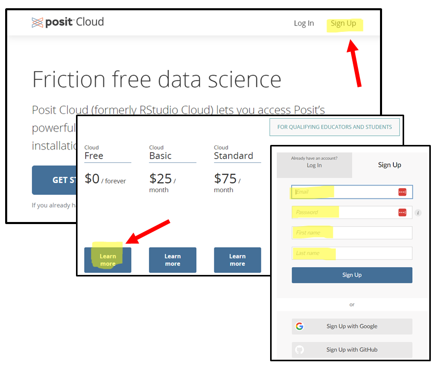
• Prove Your Worth: After submitting your details, a pigeon (or was it an email?) will fly into your inbox carrying a secret message. Click the link within to prove you’re not a goblin in disguise.

Step 2: Entering the Secret Workshop Chamber

• Return to the Portal: With your email now verified, make your way back to the RStudio Cloud realm and use your newly forged credentials to enter.

• Finding the Secret Door: One day before the workshop, a link leading to the workshop’s chamber will be sent to your e-mail.

Step 3: Joining the Fellowship of the Project

• Locate the Treasure Chest: Within the grand chamber (workshop space), seek the project “PopGenR” and click on it to reveal its secrets. As you open it for the first time, ancient RStudio Cloud spirits will work their magic to prepare your environment.

dartR fundamentals

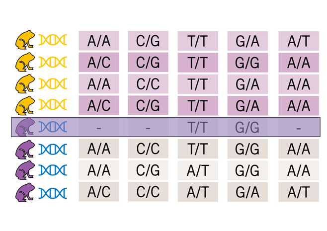
The structure of a genlight object

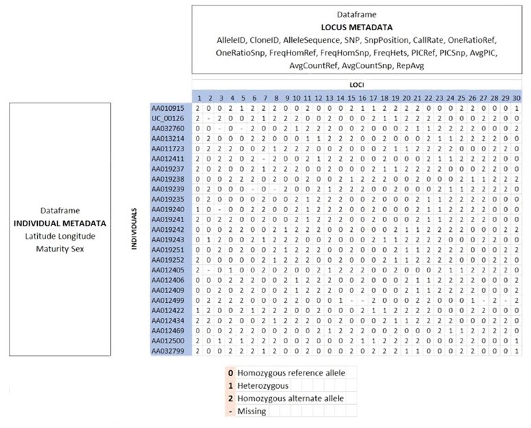
For a detailed rundown of the genetic data used by the dartRverse, check out the tutorial on Data Structure and Input found in the dartR Tutorials section.

the Basics

Here is a glimpse at the functions we will be using. Please follow along, or try running the code on your own.

code

testset.gl

gl <- testset.gl
nInd(gl)
nLoc(gl)
nPop(gl)
popNames(gl)
indNames(gl)
locNames(gl)
table(pop(gl))
as.matrix(gl)[1:7,1:5]

genlight

testset.gl

 /// GENLIGHT OBJECT /////////

 // 250 genotypes,  255 binary SNPs, size: 752 Kb
 7868 (12.34 %) missing data

 // Basic content
   @gen: list of 250 SNPbin
   @ploidy: ploidy of each individual  (range: 2-2)

 // Optional content
   @ind.names:  250 individual labels
   @loc.names:  255 locus labels
   @loc.all:  255 alleles
   @position: integer storing positions of the SNPs
   @pop: population of each individual (group size range: 1-11)
   @other: a list containing: loc.metrics  latlong  ind.metrics  history  loc.metrics.flags 

Quiz!

This quiz is referring to the testset.gl data set you have interrogated above.

Type the correct number into the blank boxes below:

• number of SNPs
• number of individuals
• number of populations

boxes will go green if you have the answer correct

Reporting and Filtering

code

gl.set.verbosity(3)

gl.report.callrate(gl)               # loci callrate             
gl.report.callrate(gl,method="ind")  # individual callrate
gl.report.reproducibility(gl)        # reproducibility

# filter
gl.filter.callrate(gl,method ="ind", threshold=0.8)

loci callrate

gl.report.callrate(gl)

Starting gl.report.callrate 
  Processing genlight object with SNP data
  Reporting Call Rate by Locus
  No. of loci = 255 
  No. of individuals = 250 
    Minimum      :  0.056 
    1st quartile :  0.912 
    Median       :  0.984 
    Mean         :  0.8765804 
    3r quartile  :  1 
    Maximum      :  1 
    Missing Rate Overall:  0.1234 

Completed: gl.report.callrate 

individual callrate

gl.report.callrate(gl,method="ind")

Starting gl.report.callrate 
  Processing genlight object with SNP data

  Reporting Call Rate by Individual
  No. of loci = 255 
  No. of individuals = 250 
    Minimum      :  0.7490196 
    1st quartile :  0.8666667 
    Median       :  0.8823529 
    Mean         :  0.8765804 
    3r quartile  :  0.8941176 
    Maximum      :  0.9333333 
    Missing Rate Overall:  0.1234 

Listing 30 populations and their average CallRates
  Monitor again after filtering
         Population CallRate  N
1     EmmacBrisWive   0.8839 10
2     EmmacBurdMist   0.8808 10
3     EmmacBurnBara   0.8859 11
4     EmmacClarJack   0.8596  5
5     EmmacClarYate   0.8769  5
6     EmmacCoopAvin   0.7682 10
7    EmmacCoopCully   0.9122 10
8     EmmacCoopEulb   0.8702 10
9    EmmacFitzAllig   0.8973 10
10    EmmacJohnWari   0.8929 10
11    EmmacMaclGeor   0.8806 11
12    EmmacMaryBoru   0.8843  6
13    EmmacMaryPetr   0.8892  4
14     EmmacMDBBowm   0.8824 10
15     EmmacMDBCond   0.8855 10
16     EmmacMDBCudg   0.8878 10
17     EmmacMDBForb   0.8766 11
18     EmmacMDBGwyd   0.9050  9
19     EmmacMDBMaci   0.8773 10
20 EmmacMDBMurrMung   0.8890 10
21     EmmacMDBSanf   0.8914 10
22    EmmacNormJack   0.8725  6
23    EmmacNormLeic   0.8863  1
24    EmmacNormSalt   0.8706  1
25    EmmacRichCasi   0.8757 10
26        EmmacRoss   0.8706 10
27    EmmacRussEube   0.8612 10
28     EmmacTweeUki   0.8773 10
29    EmsubRopeMata   0.8345  5
30    EmvicVictJasp   0.8361  5

Listing 20 individuals with the lowest CallRates
  Use this list to see which individuals will be lost on filtering by individual
  Set ind.to.list parameter to see more individuals
   Individual  CallRate
1    AA063722 0.7490196
2    AA063726 0.7490196
3    AA063732 0.7647059
4    AA063720 0.7686275
5    AA063712 0.7686275
6    AA063708 0.7725490
7    AA063718 0.7764706
8    AA063710 0.7764706
9    AA063714 0.7764706
10   AA063716 0.7803922
11   AA032760 0.7960784
12   UC_00210 0.8196078
13   UC_00259 0.8196078
14   AA018494 0.8235294
15   UC_00206 0.8235294
16   AA019164 0.8274510
17   UC_00209 0.8313725
18   UC_00254 0.8313725
19   AA019159 0.8352941
20  UC_00126c 0.8352941

)

Completed: gl.report.callrate 

reproducibility

gl.report.reproducibility(gl)

Starting gl.report.reproducibility 
  Processing genlight object with SNP data
  Reporting Repeatability by Locus
  No. of loci = 255 
  No. of individuals = 250 
    Minimum      :  0.959459 
    1st quartile :  1 
    Median       :  1 
    Mean         :  0.9981525 
    3r quartile  :  1 
    Maximum      :  1 
    Missing Rate Overall:  0.12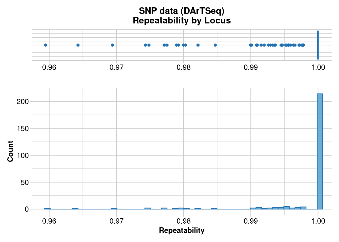 

   Quantile Threshold Retained Percent Filtered Percent
1      100%  1.000000      214    83.9       41    16.1
2       95%  1.000000      214    83.9       41    16.1
3       90%  1.000000      214    83.9       41    16.1
4       85%  1.000000      214    83.9       41    16.1
5       80%  1.000000      214    83.9       41    16.1
6       75%  1.000000      214    83.9       41    16.1
7       70%  1.000000      214    83.9       41    16.1
8       65%  1.000000      214    83.9       41    16.1
9       60%  1.000000      214    83.9       41    16.1
10      55%  1.000000      214    83.9       41    16.1
11      50%  1.000000      214    83.9       41    16.1
12      45%  1.000000      214    83.9       41    16.1
13      40%  1.000000      214    83.9       41    16.1
14      35%  1.000000      214    83.9       41    16.1
15      30%  1.000000      214    83.9       41    16.1
16      25%  1.000000      214    83.9       41    16.1
17      20%  1.000000      214    83.9       41    16.1
18      15%  0.997674      217    85.1       38    14.9
19      10%  0.994536      230    90.2       25     9.8
20       5%  0.984694      243    95.3       12     4.7
21       0%  0.959459      255   100.0        0     0.0
Completed: gl.report.reproducibility 

filter callrate

gl.filter.callrate(gl,method ="ind", threshold=0.8)

Starting gl.filter.callrate 
  Processing genlight object with SNP data
  Warning: Data may include monomorphic loci in call rate 
                    calculations for filtering
  Recalculating Call Rate
  Removing individuals based on Call Rate, threshold = 0.8 
  Individuals deleted (CallRate <=  0.8 ):
AA032760[EmmacMDBMaci], AA063718[EmmacCoopAvin], AA063720[EmmacCoopAvin], AA063722[EmmacCoopAvin], AA063726[EmmacCoopAvin], AA063732[EmmacCoopAvin], AA063708[EmmacCoopAvin], AA063710[EmmacCoopAvin], AA063712[EmmacCoopAvin], AA063714[EmmacCoopAvin], AA063716[EmmacCoopAvin],
  Summary of filtered dataset
    Call Rate for individuals > 0.8 
    Original No. of loci : 255 
    Original No. of individuals: 250 
    No. of loci retained: 255 
    No. of individuals retained: 239 
    No. of populations:  29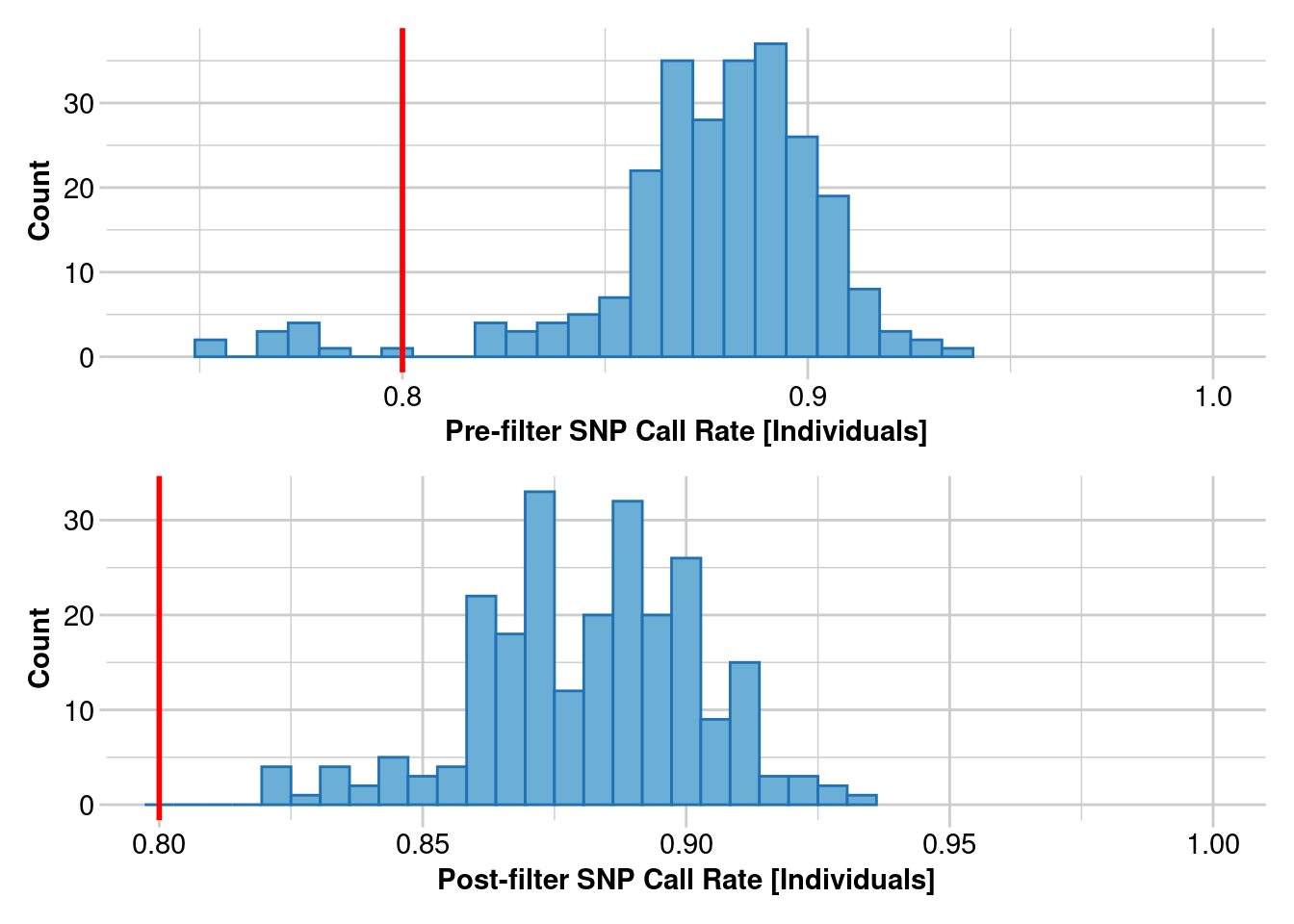 

  Note: Locus metrics not recalculated
  Note: Resultant monomorphic loci not deleted
Completed: gl.filter.callrate 

Tip

Remember, you can always look up the help file for dartRverse functions by putting a question mark (?) before a function. For example: ?gl.filter.callrate

Make sure you have the associated library loaded (eg. libary(dartR.base))

Now, lets take a look at our genetic data before and after filtering using the gl.smearplot() function.

code

gl <- testset.gl
gl.smearplot(gl) # Before Filtering

gl <- gl.filter.callrate(gl,verbose=0)
gl <- gl.filter.callrate(gl, method= "ind", 
                         threshold=0.80, verbose=0)
gl.smearplot(gl) # After Filtering

Before

  Processing genlight object with SNP data
Starting gl.smearplot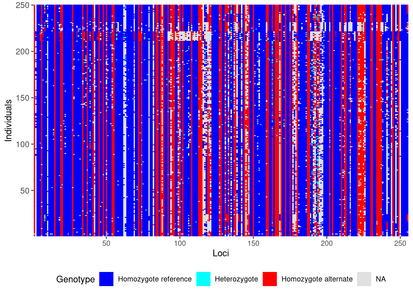 

Completed: gl.smearplot 

After

  Processing genlight object with SNP data
Starting gl.smearplot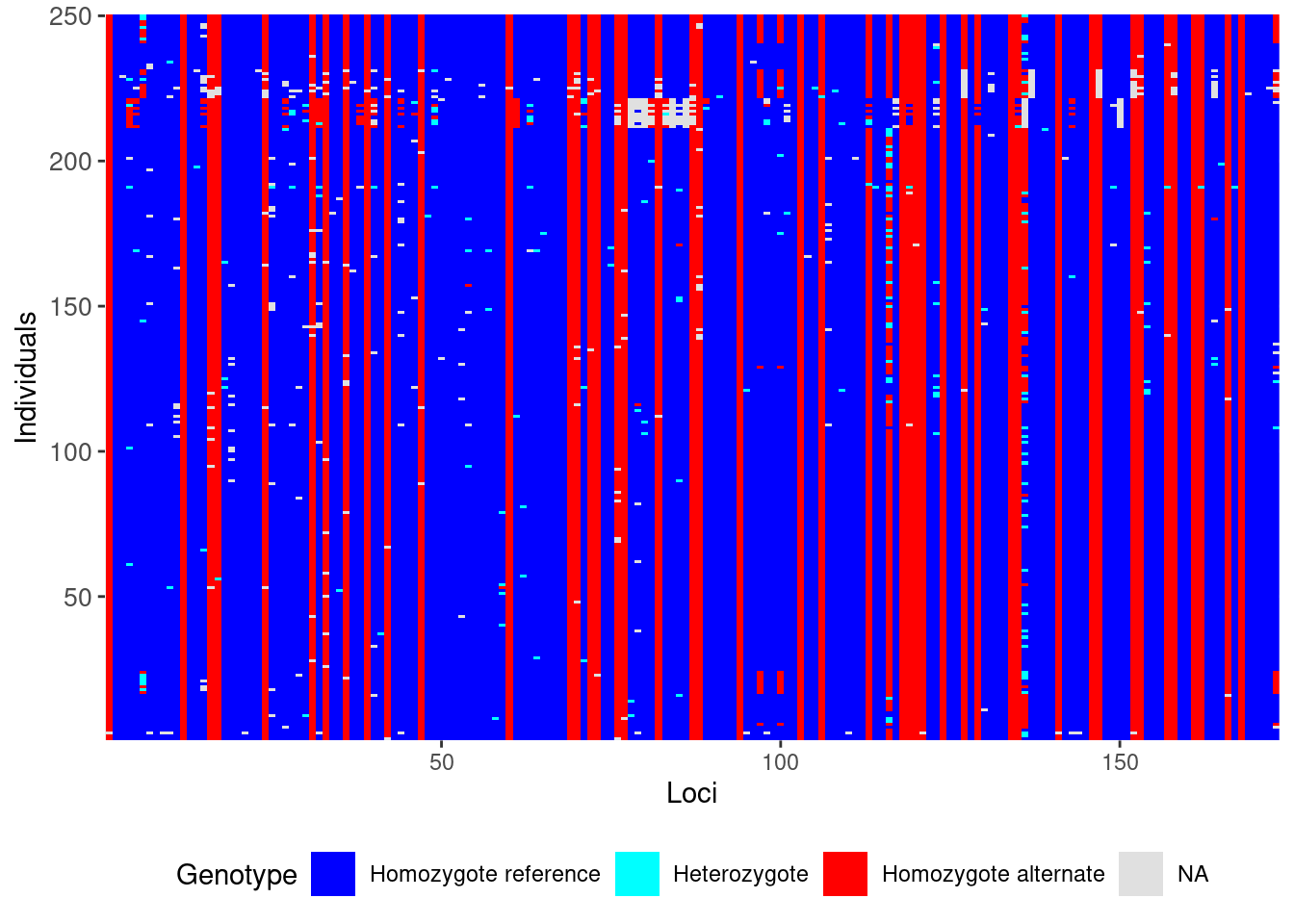 

Completed: gl.smearplot 

Filtering strategies

There is no right filtering order. Your data set will need its own interrogation, so be iterative - test different options. In some cases you may even need to reuse a filter that you used earlier on in the filtering process.

Instead of providing a recipe to follow, I recommend strategies to filtering.

First, lets have a closer look at what some of these filters do (click across the tabs for more insight into each filter):

Filters

gl.filter.callrate(method = loc) # Call rate by loci (SNPs)
gl.filter.callrate(method = ind) # Call rate by individuals
gl.filter.reproducibility()      # reproducibility 
gl.filter.rdepth()               # read depth 
gl.filter.maf()                  # minor allele frequency 
gl.filter.secondaries()          # secondaries 

callrate: loc

gl.filter.callrate(gl, method = "loc", threshold = 0.95)

What is it? Removes SNPs with too much missing data based on a specified threshold.

Why is it important? Missing loci can add “noise” and computation time to an analysis

Key Considerations:

• Trade-off between strength of filter and number of loci
• Call rate filters matter for different metrics

callrate: ind

gl.filter.callrate(gl, method = "ind", threshold = 0.95)

What is it? Removes individuals with too much missing data based on a specified threshold.

Why is it important? Deletes the key thing you need to do a study, and removes individuals that may be misleading as they are sequencing outliers

Key Considerations:

• The filtering step that costs you the very most amount of money
• Generally not a first step – recommend filtering lightly here in the first go and seeing if other filters improve the individuals completeness

reproducibility

gl.filter.reproducibility()

What is it? Diversity Arrays duplicates individuals during library prep, to assess whether the same answer is found for every locus ~ a control.

Why is it important? Provides confidence in your base calls which is pretty fundamental

Key Considerations:

• If reproducibility is low, you need your SNPs re-assessed
• If doing sequencing through AGRF or other facilities, make sure to include duplicated individuals (this is an additional cost but do it anyway)

rdepth

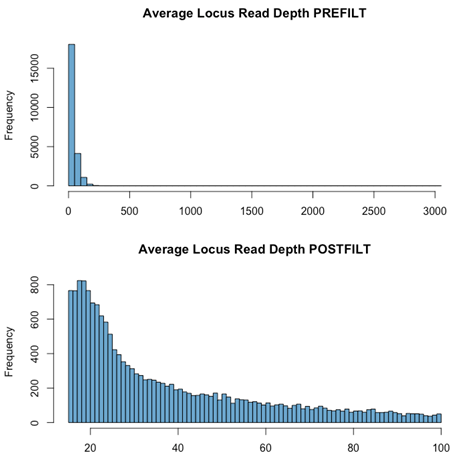
gl.filter.rdepth()

What is it? The mean number of sequencing reads for a particular locus, across all individuals.

Why is it important? The number of reads in a stack tells you how confident you can be in your base calls and a low read depth means that your heterozygous sites have pretty low coverage.

Key Considerations:

• If your read depth is not high enough, there are questions you can’t confidently answer (e.g., heterozygosity)
• Very high read depth suggests paralogs (genes with multiple copies) being assembled in to one fragment

maf

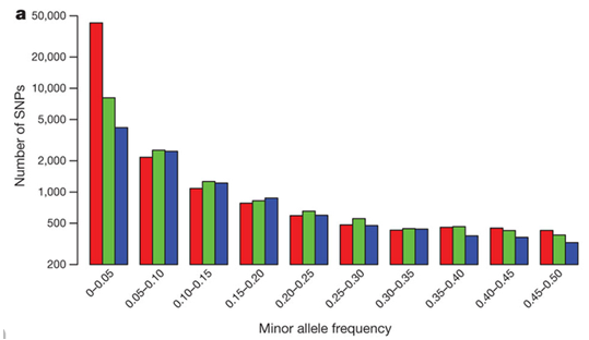
gl.filter.maf()

What is it? Minor allele frequency (maf) is the frequency of the second most common allele in a given population, so this filter removes SNPs based on their relative proportion.

Importantly, in the literature, it is often set to 0.05 BUT…

Key Considerations:

• 0.05 can be high if you have lot of individuals
  • If you have 300 diploid individuals, then you delete SNPs with less than 30 copies of the minor allele
• Or singleton if you have a small number of individuals
• Should depend on your question
  • Rare alleles can be very important to certain questions
  • Most SNPs are rare alleles, as are most heterozygous sites
  • Rare alleles are important in expansion processes
  • NOT important in structure or phylogenetic analyses

secondaries

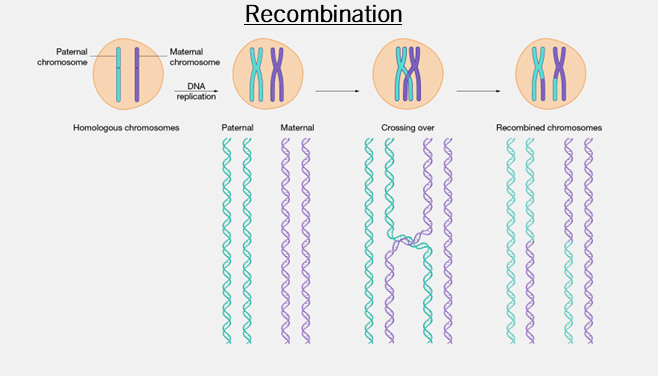
gl.filter.secondaries()

What is it? When there are two SNPs on a single fragment, choosing to keep only one.

Why is it important? Loci that are very close together in the genome are not independently inherited as they are too close together for recombination to split, so they tend to be inherited together.

Key Considerations:

• Can mislead structure and phylogenetic analyses
• Can improve representations of heterozygosity

Strategies

Now for some strategies,

as a starting point I would get rid of loci I don’t believe in and then individuals that didn’t work properly at all:

gl <- platypus.gl # example data from dartR.data

gl <- gl.filter.callrate(gl, method = "loc", threshold = 0.7)
# Get rid of really poorly sequenced loci, but don’t cut hard

gl <- gl.filter.callrate(gl, method = "ind", threshold = 0.25)
# Very low filter – this is only to get rid of your really bad 
# individuals

gl <- gl.filter.monomorphs(gl)
# Always run this after removing individuals – removes loci that are no
# longer variable

gl <- gl.filter.reproducibility(gl)
# Get rid of unreliable loci

gl <- gl.filter.rdepth(gl, lower = 5, upper = 500)
# Get rid of low and super high read depth loci

Then I would filter more strongly as appropriate for my question. For a population structure analysis I would,

gl <- gl.filter.callrate(gl, method = "loc", threshold = 0.95)
# Structure dislikes missing data

gl <- gl.filter.maf(gl,  threshold = 1/(2*nInd(gl)))
# I usually set up the threshold so it is just removing singletons to
# improve computation time

gl <- gl.filter.secondaries(gl)
# Always do this as the last loci filter so that you’ve cut for quality
# before you cut because there are two SNPs

gl <- gl.filter.callrate(gl, method = "ind", threshold = .9)
# Filter on individuals. You can usually be a bit flexible at this 
# point.

gl <- gl.filter.monomorphs(gl)
# Always run this after removing individuals

More tips

Keep these tips in mind when you go to filter your own data:

• Be flexible
• Know what each filter is doing to your data
• Think carefully about whether the filter is appropriate to the test you want to run
• Analyse your data many different ways
• Don’t over-interpret your PCoA

Exploring functions

Exercise

Try some of these report, subset, and filtering functions on your own.

Reporting

gl.report.callrate()
gl.report.reproducibility()
gl.report.secondaries()
gl.report.rdepth()
gl.report.monomorphs()
gl.report.overhang()
gl.report.hamming()
gl.report.overshoot()

Subsetting

gl.keep.ind()
gl.drop.ind()
gl.keep.loc()
gl.drop.loc()
gl.keep.pop()
gl.drop.pop()
gl.merge.pop()
gl.subsample.ind()
gl.subsample.loc()

filtering

gl.filter.callrate()
gl.filter.reproducibility()
gl.filter.secondaries()
gl.filter.rdepth()
gl.filter.monomorphs()
gl.filter.overhang()
gl.filter.hamming()
gl.filter.overshoot()

Further Study

For more tuturials see the dartR Tutorials section.

Readings

Gruber et al. (2018)

Mijangos et al. (2022)

Jaya et al. (2022)

Sopniewski and Catullo (2024)

Gruber, Bernd, Peter J. Unmack, Oliver F. Berry, and Arthur Georges. 2018. “DARTR : An R Package to Facilitate Analysis of SNP Data Generated from Reduced Representation Genome Sequencing.” Molecular Ecology Resources 18 (3): 691–99. https://doi.org/10.1111/1755-0998.12745.

Jaya, Frederick R., Jessie C. Tanner, Michael R. Whitehead, Paul Doughty, J. Scott Keogh, Craig C. Moritz, and Renee A. Catullo. 2022. “Population Genomics and Sexual Signals Support Reproductive Character Displacement in Uperoleia (Anura: Myobatrachidae) in a Contact Zone.” Molecular Ecology 31 (17): 4527–43. https://doi.org/10.1111/mec.16597.

Mijangos, Jose Luis, Bernd Gruber, Oliver Berry, Carlo Pacioni, and Arthur Georges. 2022. “dartR V2: An Accessible Genetic Analysis Platform for Conservation, Ecology and Agriculture.” Methods in Ecology and Evolution 13 (10): 2150–58. https://doi.org/10.1111/2041-210X.13918.

Sopniewski, Jarrod, and Renee A. Catullo. 2024. “Estimates of Heterozygosity from Single Nucleotide Polymorphism Markers Are Context-Dependent and Often Wrong.” Molecular Ecology Resources, March, e13947. https://doi.org/10.1111/1755-0998.13947.