library(dartRverse)
library(ggplot2)3 Sequencing Technologies
Session Presenters

Required packages
make sure you have the packages installed, see Install dartRverse
DArT sequencing
![]()

DArTseq is our proprietary genome complexity reduction-based sequencing technology.
It differs from other methods through its ability to intelligently select the predominantly active – low copy sequence – areas in a genome, which are the ones containing the most useful information. At the same time, DArTseq masks the lesser value, repetitive sequences. It does this through the application of a combination of restriction enzymes to fragment DNA samples in a highly reproducible manner.
A key component of DArTseq is its complexity reduction step. This involves reducing complexity of the genome by cutting it down to a consistent and reproducible fraction from which markers are discovered and called. This process does not introduce ascertainment bias because we are discovering markers within the (restriction) fragment set without the bias.
Characteristics
DArTseq is designed to provide a consistent genomic representation across samples within and between experiments, even over a decade of operations. DArTseq has been used to process tens of thousands of samples from hundreds of organisms, and is capable of co-analysing thousands of samples together, with the great majority of markers called across all of the samples. These advantages come from the library processing methods of DArTseq which distinguish it from all other complexity reduced genotyping technologies using restriction enzymes.
Standardised
Laboratory sample processing is performed in a very high throughput streamlined operation utilising end-to-end pipetting robotics and informatics integration, with a Laboratory Information Management System (LIMS). All the physical sample processing steps undertaken in the lab are linked with the data storage and analysis components via tight integration with the LIMS. Sample processing robots have automated data exchange with the LIMS.
Manual operations have been minimised and plate based sample handling prevents the introduction of sample-tracking mistakes after arrival. The analytical components for processing DArTseq data and generating marker calls have been tailored specifically to the unique DArTseq complexity reduction and library construction methods. This results in a streamlined and highly effective data analysis pipeline, enabling rapid generation of high-quality marker data from thousands or even tens of thousands of assays in a single analysis. Ability to co-analysis with past services of 14 years despite 5 generations of the illumina sequences. The population of fragments in the genomic representation does not vary across multiple sample submissions despite the many years.
See more at https://www.diversityarrays.com/
SNP-based heterozygosity estimates
1. Estimating heterozygosity: 70% callrate
How do estimates of heterozygosity change as the number of individuals changes in your SNP calling?
This uses data from Litoria rubella, a very abundant and widespread frog species. We are using data following https://onlinelibrary.wiley.com/doi/10.1111/1755-0998.13947. Let’s focus on the Kimberley, where we have lots of samples, and we expect the diversity to be really high because there are millions of them everywhere. SNPs were called on different numbers of individuals, in increments of 5 using the Stacks pipeline. We are only going to do a simple filter for call rates because we already filtered for allele depth in Stacks. SNPs were called independent of other populations, which we will get to later.
Load data
# load data
load('./data/Session3_data.RData')

#create a list of the kimberley genlights
kimberley_names <- ls(pattern = "^Kimberley")
#put all the genlights into a mega list
kimberley <- mget(kimberley_names)

#we're going to do this in a loop for speed, applying the same filters
# Iterate over the names of the kimberley list
for(name in names(kimberley)){
  # Extract the genlight object from the kimberley list using its name
  genlight_object <- kimberley[[name]]
  # Apply the filter call rate function
  # Assuming gl.filter.callrate is a function that operates on a genlight object
  filtered_object <- gl.filter.callrate(genlight_object, threshold = 0.7, mono.rm = TRUE)
  # Assign the filtered object back to the environment with a new name
  assign(paste0(name, "_0.7"), filtered_object)
}
Starting gl.filter.callrate
Processing genlight object with SNP data
Warning: data include loci that are scored NA across all individuals.
Consider filtering using gl <- gl.filter.allna(gl)
Warning: Data may include monomorphic loci in call rate
calculations for filtering
Recalculating Call Rate
Removing loci based on Call Rate, threshold = 0.7 
Completed: gl.filter.callrate
Starting gl.filter.callrate
  Processing genlight object with SNP data
  Warning: data include loci that are scored NA across all individuals.
  Consider filtering using gl <- gl.filter.allna(gl)
  Warning: Data may include monomorphic loci in call rate
                    calculations for filtering
  Recalculating Call Rate
Removing loci based on Call Rate, threshold = 0.7 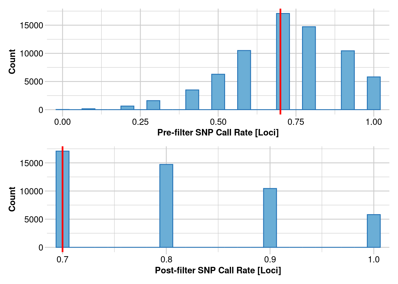
Completed: gl.filter.callrate
Starting gl.filter.callrate
  Processing genlight object with SNP data
  Warning: Data may include monomorphic loci in call rate
                    calculations for filtering
  Recalculating Call Rate
Removing loci based on Call Rate, threshold = 0.7 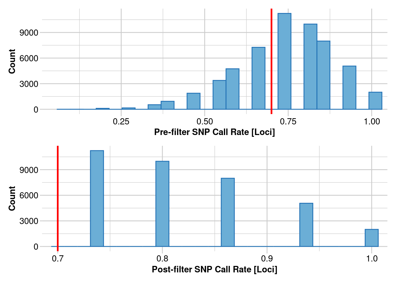
Completed: gl.filter.callrate
Starting gl.filter.callrate
  Processing genlight object with SNP data
  Warning: Data may include monomorphic loci in call rate
                    calculations for filtering
  Recalculating Call Rate
Removing loci based on Call Rate, threshold = 0.7 
Completed: gl.filter.callrate
Starting gl.filter.callrate
  Processing genlight object with SNP data
  Warning: Data may include monomorphic loci in call rate
                    calculations for filtering
  Recalculating Call Rate
Removing loci based on Call Rate, threshold = 0.7 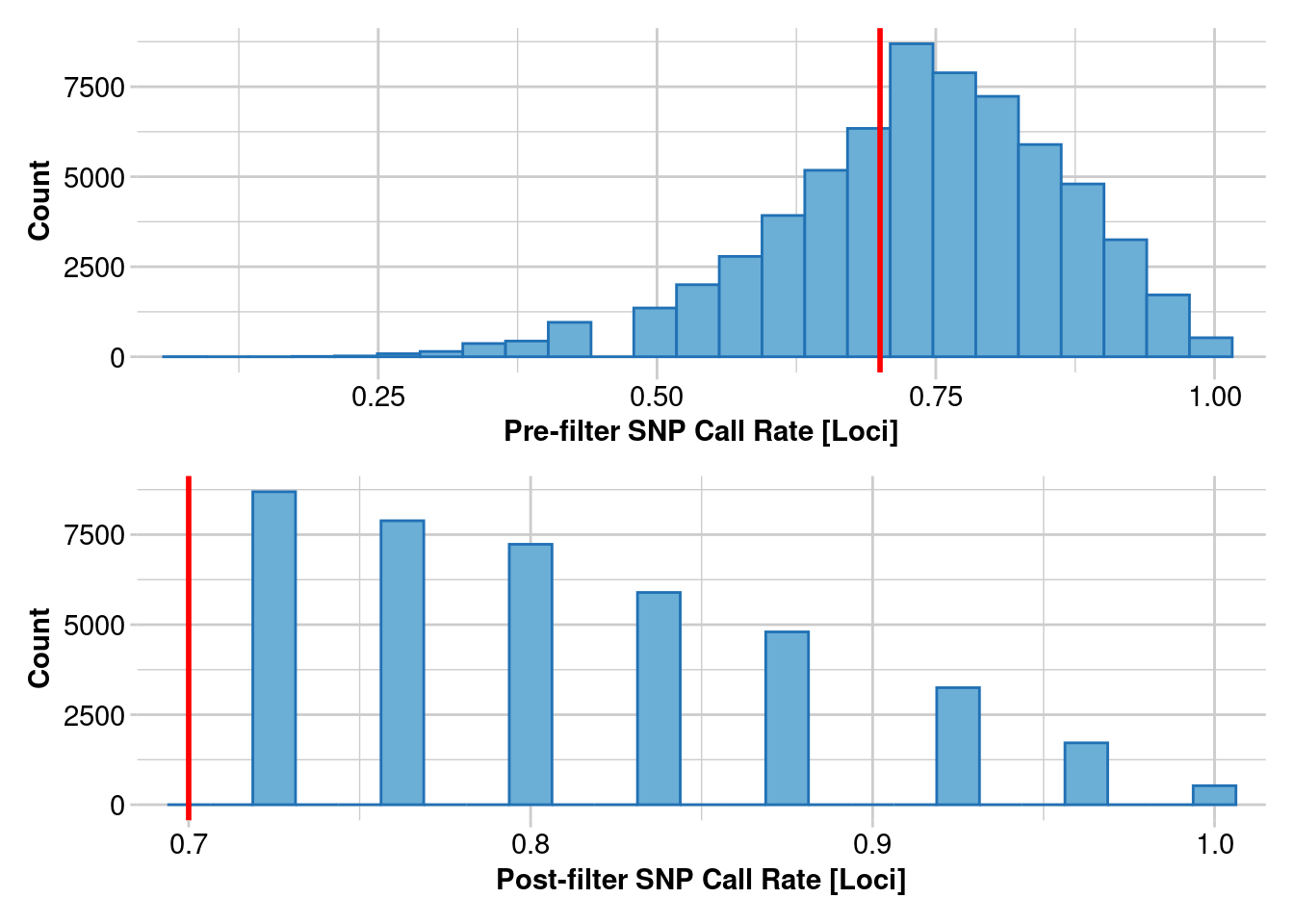
Completed: gl.filter.callrate
Starting gl.filter.callrate
  Processing genlight object with SNP data
  Warning: Data may include monomorphic loci in call rate
                    calculations for filtering
  Recalculating Call Rate
Removing loci based on Call Rate, threshold = 0.7 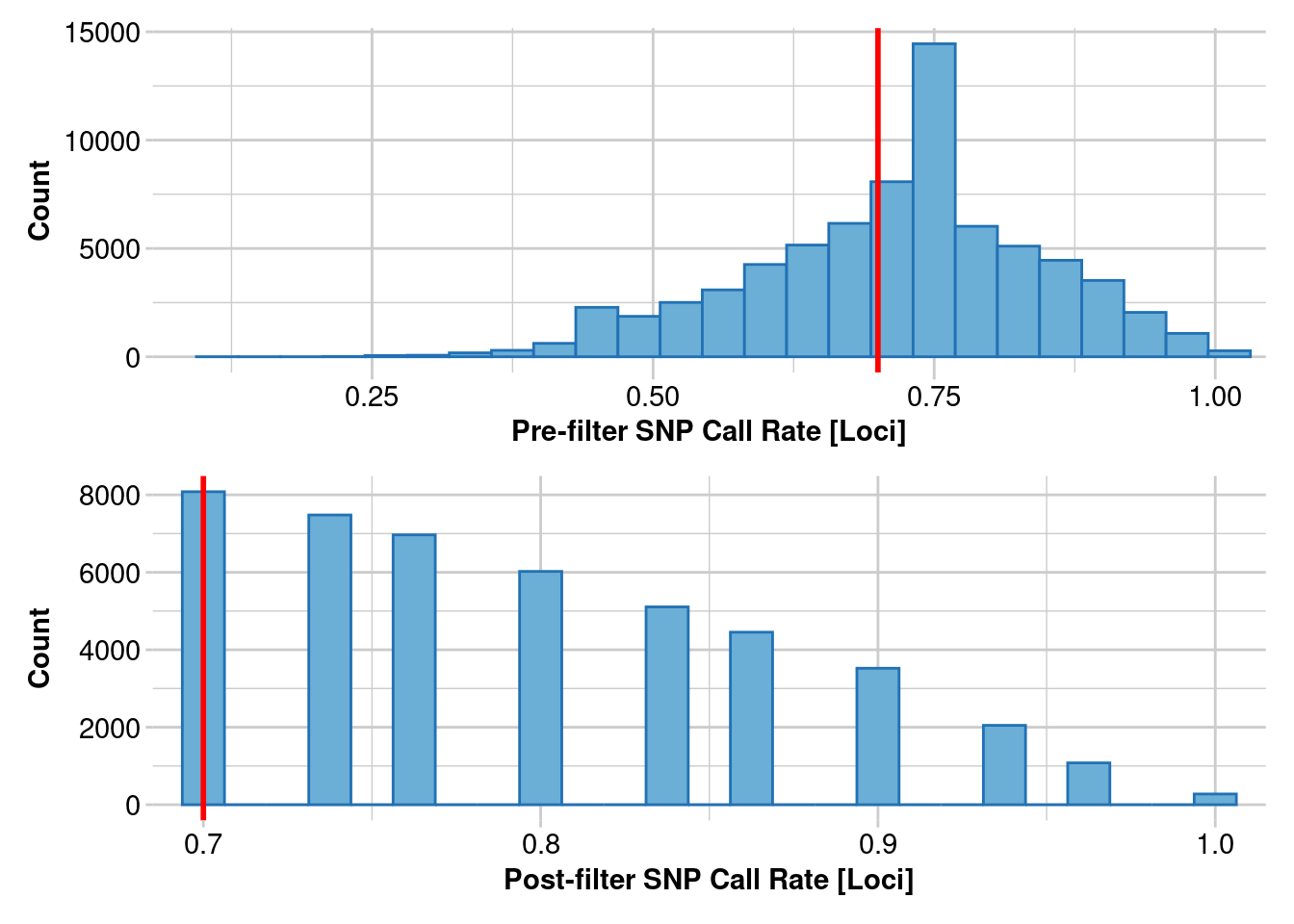
Completed: gl.filter.callrate
Starting gl.filter.callrate
  Processing genlight object with SNP data
  Warning: Data may include monomorphic loci in call rate
                    calculations for filtering
  Recalculating Call Rate
Removing loci based on Call Rate, threshold = 0.7 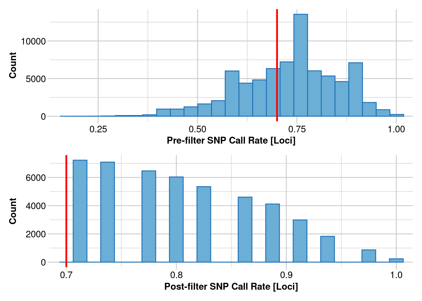
Completed: gl.filter.callrate
Starting gl.filter.callrate
  Processing genlight object with SNP data
  Warning: Data may include monomorphic loci in call rate
                    calculations for filtering
  Recalculating Call Rate
Removing loci based on Call Rate, threshold = 0.7 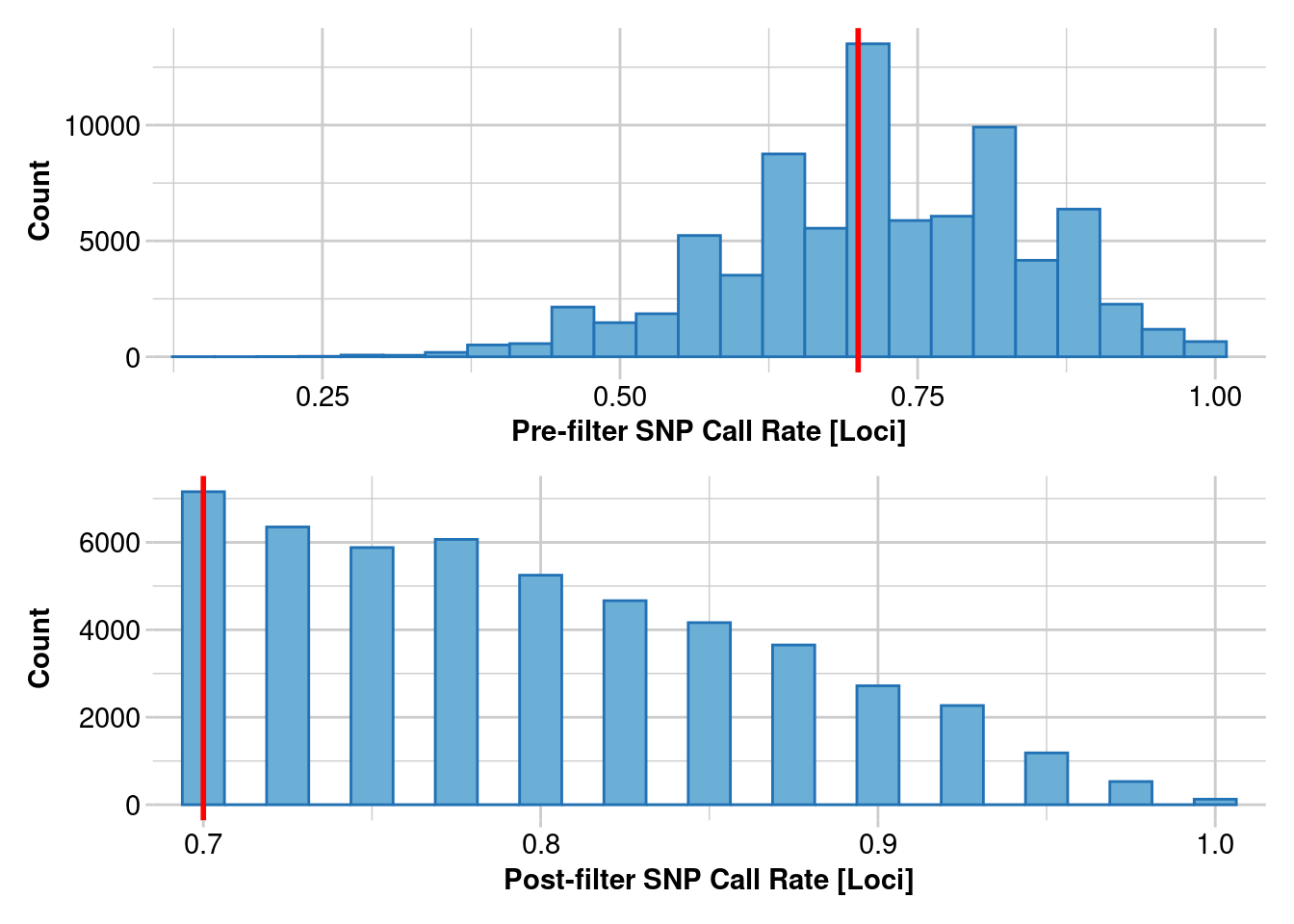
Completed: gl.filter.callrate Calculate heterozygosity
# List all object names in the environment
all_names <- ls()

# Use grep() to match names that start with "Kimberley"
# and end with "0.7", .+ indicates any characters in between
kimberley_filtered <- grep("^Kimberley.+0\\.7$", all_names, value = TRUE)#put all the genlights into a mega list
#create another list with the ones we want
kimberley <- mget(kimberley_filtered)

#Initialize an empty data frame
heterozygosity_reports_df <- data.frame()

# Iterate over the kimberley list to apply gl.report.heterozygosity
# and bind the results
for(name in names(kimberley)) {
  # Apply the function
  report <- gl.report.heterozygosity(kimberley[[name]])

  # Add 'ObjectName' as the first column of the report
  report <- cbind(ObjectName = name, report)

  # Bind this report to the main data frame
  heterozygosity_reports_df <- bind_rows(heterozygosity_reports_df, report)
}
Starting gl.report.heterozygosity
Processing genlight object with SNP data
Calculating Observed Heterozygosities, averaged across
loci, for each population
Calculating Expected Heterozygosities
Starting gl.colors
Selected color type dis
Completed: gl.colors 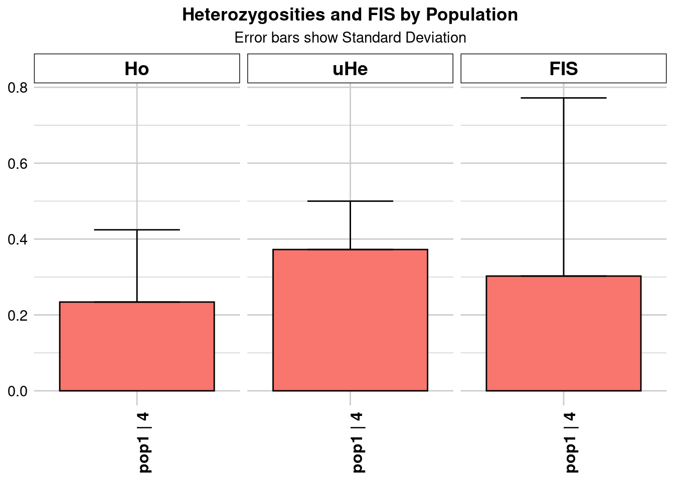
pop n.Ind n.Loc n.Loc.adj polyLoc monoLoc all_NALoc Ho HoSD
pop1 pop1 4.327947 28465 1 28465 0 0 0.233986 0.190371
HoSE HoLCI HoHCI Ho.adj Ho.adjSD Ho.adjSE Ho.adjLCI Ho.adjHCI
pop1 0.001128 NA NA 0.233986 0.190371 0.001128 NA NA
He HeSD HeSE HeLCI HeHCI uHe uHeSD uHeSE uHeLCI
pop1 0.329375 0.112778 0.000668 NA NA 0.372398 0.127509 0.000756 NA
uHeHCI He.adj He.adjSD He.adjSE He.adjLCI He.adjHCI FIS FISSD
pop1 NA 0.329375 0.112778 0.000668 NA NA 0.302454 0.469498
FISSE FISLCI FISHCI
pop1 0.002783 NA NA
Completed: gl.report.heterozygosity
Starting gl.report.heterozygosity
  Processing genlight object with SNP data
  Calculating Observed Heterozygosities, averaged across
                    loci, for each population
  Calculating Expected Heterozygosities

Starting gl.colors
Selected color type dis
Completed: gl.colors 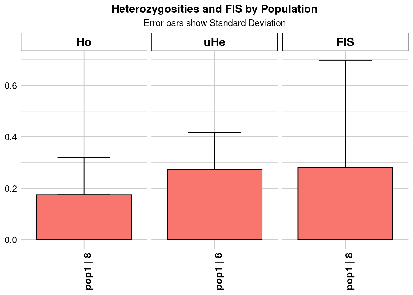
      pop    n.Ind n.Loc n.Loc.adj polyLoc monoLoc all_NALoc       Ho     HoSD
pop1 pop1 8.113689 47375         1   47375       0         0 0.174677 0.144488
         HoSE HoLCI HoHCI   Ho.adj Ho.adjSD Ho.adjSE Ho.adjLCI Ho.adjHCI
pop1 0.000664    NA    NA 0.174677 0.144488 0.000664        NA        NA
           He     HeSD    HeSE HeLCI HeHCI      uHe    uHeSD    uHeSE uHeLCI
pop1 0.256162 0.135015 0.00062    NA    NA 0.272985 0.143882 0.000661     NA
     uHeHCI   He.adj He.adjSD He.adjSE He.adjLCI He.adjHCI      FIS    FISSD
pop1     NA 0.256162 0.135015  0.00062        NA        NA 0.279239 0.419149
        FISSE FISLCI FISHCI
pop1 0.001926     NA     NA
Completed: gl.report.heterozygosity
Starting gl.report.heterozygosity
  Processing genlight object with SNP data
  Calculating Observed Heterozygosities, averaged across
                    loci, for each population
  Calculating Expected Heterozygosities

Starting gl.colors
Selected color type dis
Completed: gl.colors 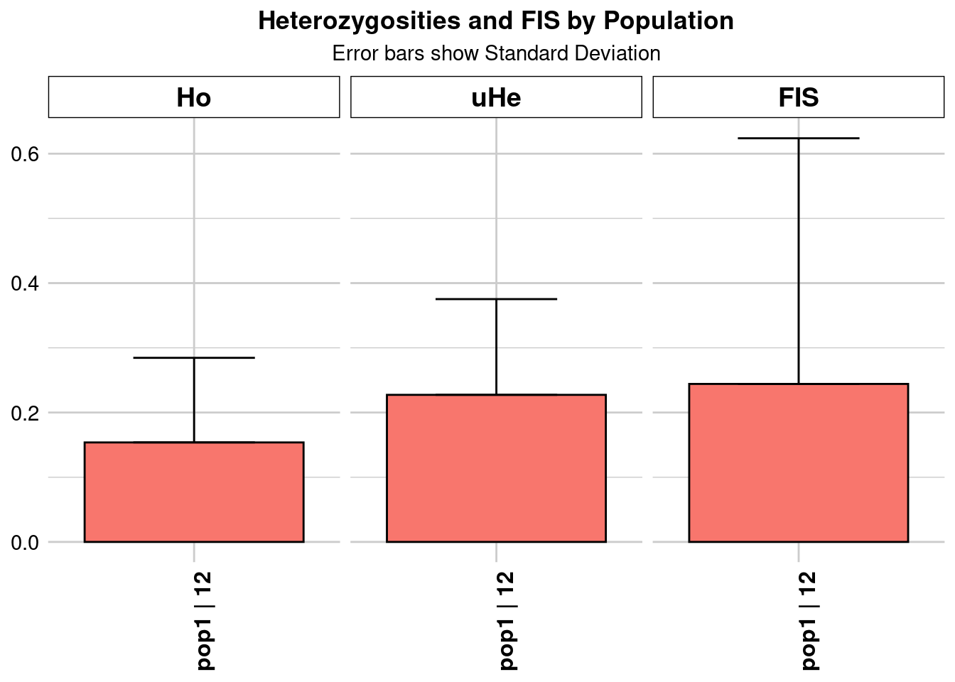
      pop    n.Ind n.Loc n.Loc.adj polyLoc monoLoc all_NALoc      Ho     HoSD
pop1 pop1 12.36041 35945         1   35945       0         0 0.15375 0.130734
        HoSE HoLCI HoHCI  Ho.adj Ho.adjSD Ho.adjSE Ho.adjLCI Ho.adjHCI       He
pop1 0.00069    NA    NA 0.15375 0.130734  0.00069        NA        NA 0.218107
        HeSD     HeSE HeLCI HeHCI      uHe    uHeSD   uHeSE uHeLCI uHeHCI
pop1 0.14199 0.000749    NA    NA 0.227301 0.147975 0.00078     NA     NA
       He.adj He.adjSD He.adjSE He.adjLCI He.adjHCI      FIS    FISSD    FISSE
pop1 0.218107  0.14199 0.000749        NA        NA 0.244173 0.379656 0.002002
     FISLCI FISHCI
pop1     NA     NA
Completed: gl.report.heterozygosity
Starting gl.report.heterozygosity
  Processing genlight object with SNP data
  Calculating Observed Heterozygosities, averaged across
                    loci, for each population
  Calculating Expected Heterozygosities

Starting gl.colors
Selected color type dis
Completed: gl.colors 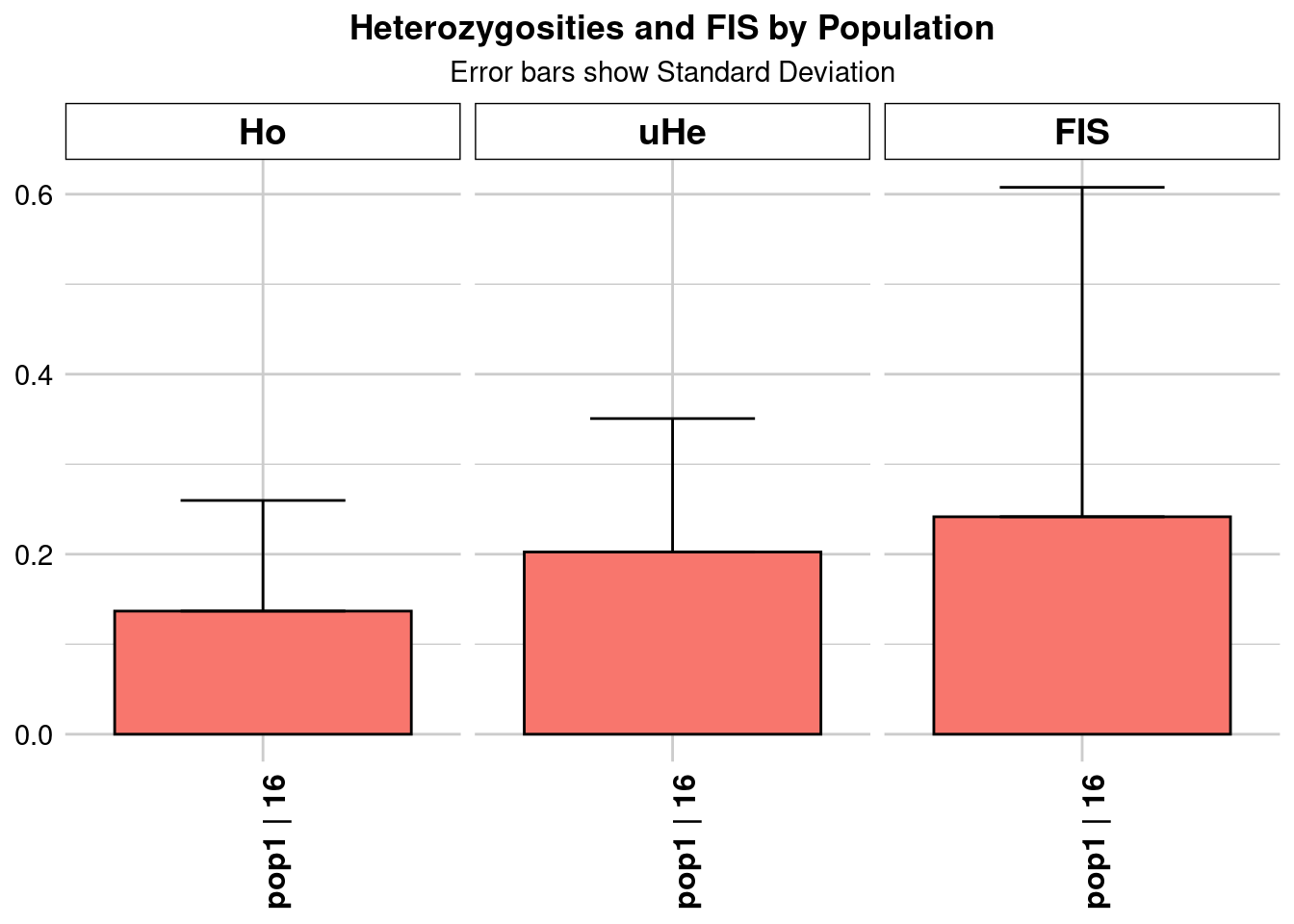
      pop    n.Ind n.Loc n.Loc.adj polyLoc monoLoc all_NALoc       Ho     HoSD
pop1 pop1 16.03257 46276         1   46276       0         0 0.136788 0.122952
         HoSE HoLCI HoHCI   Ho.adj Ho.adjSD Ho.adjSE Ho.adjLCI Ho.adjHCI
pop1 0.000572    NA    NA 0.136788 0.122952 0.000572        NA        NA
           He     HeSD     HeSE HeLCI HeHCI      uHe    uHeSD    uHeSE uHeLCI
pop1 0.196149 0.143623 0.000668    NA    NA 0.202464 0.148246 0.000689     NA
     uHeHCI   He.adj He.adjSD He.adjSE He.adjLCI He.adjHCI     FIS    FISSD
pop1     NA 0.196149 0.143623 0.000668        NA        NA 0.24159 0.366035
        FISSE FISLCI FISHCI
pop1 0.001702     NA     NA
Completed: gl.report.heterozygosity
Starting gl.report.heterozygosity
  Processing genlight object with SNP data
  Calculating Observed Heterozygosities, averaged across
                    loci, for each population
  Calculating Expected Heterozygosities

Starting gl.colors
Selected color type dis
Completed: gl.colors 
      pop    n.Ind n.Loc n.Loc.adj polyLoc monoLoc all_NALoc       Ho     HoSD
pop1 pop1 20.24648 39573         1   39573       0         0 0.128296 0.118505
         HoSE HoLCI HoHCI   Ho.adj Ho.adjSD Ho.adjSE Ho.adjLCI Ho.adjHCI
pop1 0.000596    NA    NA 0.128296 0.118505 0.000596        NA        NA
           He     HeSD     HeSE HeLCI HeHCI      uHe    uHeSD    uHeSE uHeLCI
pop1 0.180369 0.144139 0.000725    NA    NA 0.184936 0.147788 0.000743     NA
     uHeHCI   He.adj He.adjSD He.adjSE He.adjLCI He.adjHCI      FIS    FISSD
pop1     NA 0.180369 0.144139 0.000725        NA        NA 0.224197 0.345555
        FISSE FISLCI FISHCI
pop1 0.001737     NA     NA
Completed: gl.report.heterozygosity
Starting gl.report.heterozygosity
  Processing genlight object with SNP data
  Calculating Observed Heterozygosities, averaged across
                    loci, for each population
  Calculating Expected Heterozygosities

Starting gl.colors
Selected color type dis
Completed: gl.colors 
      pop    n.Ind n.Loc n.Loc.adj polyLoc monoLoc all_NALoc       Ho     HoSD
pop1 pop1 23.86971 44532         1   44532       0         0 0.122023 0.115572
         HoSE HoLCI HoHCI   Ho.adj Ho.adjSD Ho.adjSE Ho.adjLCI Ho.adjHCI
pop1 0.000548    NA    NA 0.122023 0.115572 0.000548        NA        NA
           He     HeSD     HeSE HeLCI HeHCI      uHe    uHeSD    uHeSE uHeLCI
pop1 0.172406 0.144272 0.000684    NA    NA 0.176095 0.147359 0.000698     NA
     uHeHCI   He.adj He.adjSD He.adjSE He.adjLCI He.adjHCI      FIS    FISSD
pop1     NA 0.172406 0.144272 0.000684        NA        NA 0.225027 0.336198
        FISSE FISLCI FISHCI
pop1 0.001593     NA     NA
Completed: gl.report.heterozygosity
Starting gl.report.heterozygosity
  Processing genlight object with SNP data
  Calculating Observed Heterozygosities, averaged across
                    loci, for each population
  Calculating Expected Heterozygosities

Starting gl.colors
Selected color type dis
Completed: gl.colors 
      pop    n.Ind n.Loc n.Loc.adj polyLoc monoLoc all_NALoc       Ho     HoSD
pop1 pop1 28.28105 46273         1   46273       0         0 0.114091 0.112716
         HoSE HoLCI HoHCI   Ho.adj Ho.adjSD Ho.adjSE Ho.adjLCI Ho.adjHCI
pop1 0.000524    NA    NA 0.114091 0.112716 0.000524        NA        NA
           He     HeSD     HeSE HeLCI HeHCI      uHe    uHeSD    uHeSE uHeLCI
pop1 0.160215 0.143001 0.000665    NA    NA 0.163099 0.145574 0.000677     NA
     uHeHCI   He.adj He.adjSD He.adjSE He.adjLCI He.adjHCI      FIS    FISSD
pop1     NA 0.160215 0.143001 0.000665        NA        NA 0.217536 0.325623
        FISSE FISLCI FISHCI
pop1 0.001514     NA     NA
Completed: gl.report.heterozygosity
Starting gl.report.heterozygosity
  Processing genlight object with SNP data
  Calculating Observed Heterozygosities, averaged across
                    loci, for each population
  Calculating Expected Heterozygosities

Starting gl.colors
Selected color type dis
Completed: gl.colors 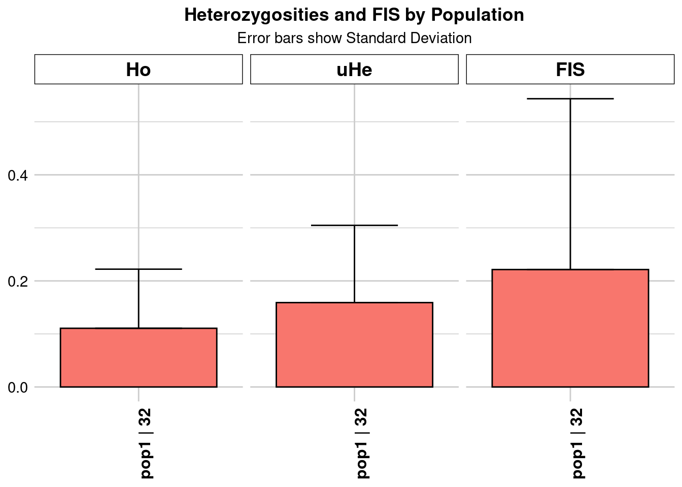
      pop    n.Ind n.Loc n.Loc.adj polyLoc monoLoc all_NALoc       Ho     HoSD
pop1 pop1 31.86356 49487         1   49487       0         0 0.110686 0.111441
         HoSE HoLCI HoHCI   Ho.adj Ho.adjSD Ho.adjSE Ho.adjLCI Ho.adjHCI
pop1 0.000501    NA    NA 0.110686 0.111441 0.000501        NA        NA
           He     HeSD     HeSE HeLCI HeHCI      uHe    uHeSD    uHeSE uHeLCI
pop1 0.156579 0.143352 0.000644    NA    NA 0.159075 0.145637 0.000655     NA
     uHeHCI   He.adj He.adjSD He.adjSE He.adjLCI He.adjHCI      FIS   FISSD
pop1     NA 0.156579 0.143352 0.000644        NA        NA 0.221427 0.32204
        FISSE FISLCI FISHCI
pop1 0.001448     NA     NA
Completed: gl.report.heterozygosity
# heterozygosity_reports_df now contains all the reports with an
# additional column for object names
knitr::kable(heterozygosity_reports_df)| ObjectName | pop | n.Ind | n.Loc | n.Loc.adj | polyLoc | monoLoc | all_NALoc | Ho | HoSD | HoSE | HoLCI | HoHCI | Ho.adj | Ho.adjSD | Ho.adjSE | Ho.adjLCI | Ho.adjHCI | He | HeSD | HeSE | HeLCI | HeHCI | uHe | uHeSD | uHeSE | uHeLCI | uHeHCI | He.adj | He.adjSD | He.adjSE | He.adjLCI | He.adjHCI | FIS | FISSD | FISSE | FISLCI | FISHCI | |
|---|---|---|---|---|---|---|---|---|---|---|---|---|---|---|---|---|---|---|---|---|---|---|---|---|---|---|---|---|---|---|---|---|---|---|---|---|---|---|
| pop1…1 | Kimberley_n_05.vcf_0.7 | pop1 | 4.327947 | 28465 | 1 | 28465 | 0 | 0 | 0.233986 | 0.190371 | 0.001128 | NA | NA | 0.233986 | 0.190371 | 0.001128 | NA | NA | 0.329375 | 0.112778 | 0.000668 | NA | NA | 0.372398 | 0.127509 | 0.000756 | NA | NA | 0.329375 | 0.112778 | 0.000668 | NA | NA | 0.302454 | 0.469498 | 0.002783 | NA | NA |
| pop1…2 | Kimberley_n_10.vcf_0.7 | pop1 | 8.113689 | 47375 | 1 | 47375 | 0 | 0 | 0.174677 | 0.144488 | 0.000664 | NA | NA | 0.174677 | 0.144488 | 0.000664 | NA | NA | 0.256162 | 0.135015 | 0.000620 | NA | NA | 0.272985 | 0.143882 | 0.000661 | NA | NA | 0.256162 | 0.135015 | 0.000620 | NA | NA | 0.279239 | 0.419149 | 0.001926 | NA | NA |
| pop1…3 | Kimberley_n_15.vcf_0.7 | pop1 | 12.360412 | 35945 | 1 | 35945 | 0 | 0 | 0.153750 | 0.130734 | 0.000690 | NA | NA | 0.153750 | 0.130734 | 0.000690 | NA | NA | 0.218107 | 0.141990 | 0.000749 | NA | NA | 0.227301 | 0.147975 | 0.000780 | NA | NA | 0.218107 | 0.141990 | 0.000749 | NA | NA | 0.244173 | 0.379656 | 0.002002 | NA | NA |
| pop1…4 | Kimberley_n_20.vcf_0.7 | pop1 | 16.032565 | 46276 | 1 | 46276 | 0 | 0 | 0.136788 | 0.122952 | 0.000572 | NA | NA | 0.136788 | 0.122952 | 0.000572 | NA | NA | 0.196149 | 0.143623 | 0.000668 | NA | NA | 0.202464 | 0.148246 | 0.000689 | NA | NA | 0.196149 | 0.143623 | 0.000668 | NA | NA | 0.241590 | 0.366035 | 0.001702 | NA | NA |
| pop1…5 | Kimberley_n_25.vcf_0.7 | pop1 | 20.246481 | 39573 | 1 | 39573 | 0 | 0 | 0.128296 | 0.118505 | 0.000596 | NA | NA | 0.128296 | 0.118505 | 0.000596 | NA | NA | 0.180369 | 0.144139 | 0.000725 | NA | NA | 0.184936 | 0.147788 | 0.000743 | NA | NA | 0.180369 | 0.144139 | 0.000725 | NA | NA | 0.224197 | 0.345555 | 0.001737 | NA | NA |
| pop1…6 | Kimberley_n_30.vcf_0.7 | pop1 | 23.869712 | 44532 | 1 | 44532 | 0 | 0 | 0.122023 | 0.115572 | 0.000548 | NA | NA | 0.122023 | 0.115572 | 0.000548 | NA | NA | 0.172406 | 0.144272 | 0.000684 | NA | NA | 0.176095 | 0.147359 | 0.000698 | NA | NA | 0.172406 | 0.144272 | 0.000684 | NA | NA | 0.225027 | 0.336198 | 0.001593 | NA | NA |
| pop1…7 | Kimberley_n_35.vcf_0.7 | pop1 | 28.281049 | 46273 | 1 | 46273 | 0 | 0 | 0.114091 | 0.112716 | 0.000524 | NA | NA | 0.114091 | 0.112716 | 0.000524 | NA | NA | 0.160215 | 0.143001 | 0.000665 | NA | NA | 0.163099 | 0.145574 | 0.000677 | NA | NA | 0.160215 | 0.143001 | 0.000665 | NA | NA | 0.217536 | 0.325623 | 0.001514 | NA | NA |
| pop1…8 | Kimberley_n_40.vcf_0.7 | pop1 | 31.863560 | 49487 | 1 | 49487 | 0 | 0 | 0.110686 | 0.111441 | 0.000501 | NA | NA | 0.110686 | 0.111441 | 0.000501 | NA | NA | 0.156579 | 0.143352 | 0.000644 | NA | NA | 0.159075 | 0.145637 | 0.000655 | NA | NA | 0.156579 | 0.143352 | 0.000644 | NA | NA | 0.221427 | 0.322040 | 0.001448 | NA | NA |
Plotting results
kimberley_Ho_0.7callrate <- ggplot(heterozygosity_reports_df, aes(x = ObjectName, y = Ho)) +
  geom_point() +
  scale_y_continuous(limits = c(0, NA)) +
  theme(axis.text.x = element_text(angle = 65, hjust = 1)) +
  labs(title = "Observed Heterozygosity by Sample number", x = "Sample Number", y = "Observed Heterozygosity (Ho) at 0.7 Call Rate")

kimberley_Ho_0.7callrate
Sampling
As you can see, different numbers of samples can substantially change your heterozygosity estimate.
2. Estimating heterozygosity: 95% callrate
Lets redo our heterozygosity estimates, but see how changing your call rate filter impacts estimates
Reload data
# reload data
load('./data/Session3_data.RData')
# List all object names in the environment
all_names <- ls()

# Use grep() to match names that start with "Kimberley"
kimberley_names <- grep("^Kimberley.*\\.vcf$", all_names, value = TRUE) #put all the genlights into a mega list
#create another list with the ones we want
kimberley <- mget(kimberley_names)

#we're going to do this in a loop for speed, applying the same filters
# Iterate over the names of the kimberley list
for(name in names(kimberley)){
  # Extract the genlight object from the kimberley list using its name
  genlight_object <- kimberley[[name]]
  # Apply the filter call rate function
  # Assuming gl.filter.callrate is a function that operates on a genlight object
   filtered_object <- gl.filter.callrate(genlight_object, threshold = .95, mono.rm = TRUE)
  # Assign the filtered object back to the environment with a new name
  assign(paste0(name, "_0.95"), filtered_object)
}
Starting gl.filter.callrate
Processing genlight object with SNP data
Warning: data include loci that are scored NA across all individuals.
Consider filtering using gl <- gl.filter.allna(gl)
Warning: Data may include monomorphic loci in call rate
calculations for filtering
Recalculating Call Rate
Removing loci based on Call Rate, threshold = 0.95 
Completed: gl.filter.callrate
Starting gl.filter.callrate
  Processing genlight object with SNP data
  Warning: data include loci that are scored NA across all individuals.
  Consider filtering using gl <- gl.filter.allna(gl)
  Warning: Data may include monomorphic loci in call rate
                    calculations for filtering
  Recalculating Call Rate
Removing loci based on Call Rate, threshold = 0.95 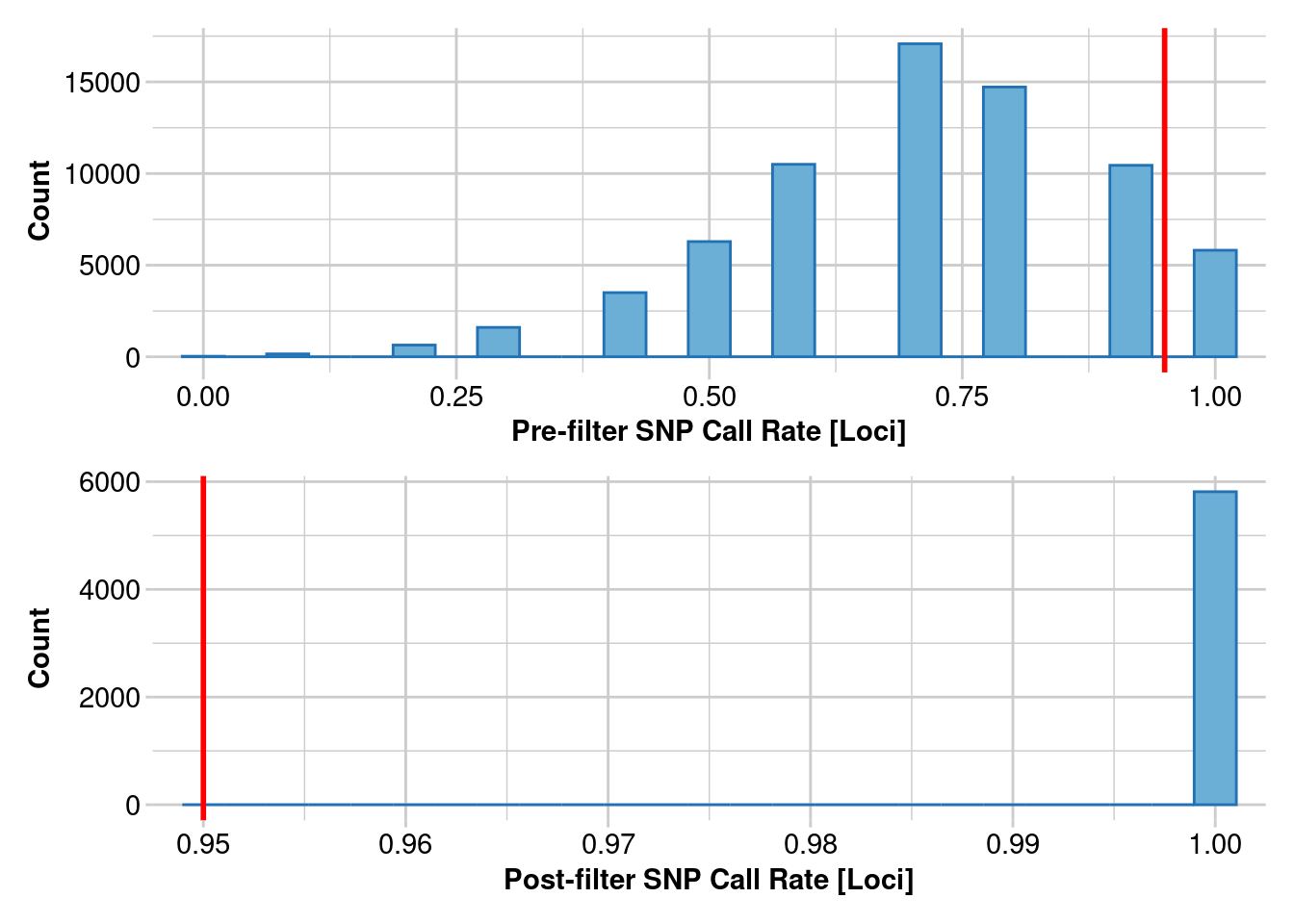
Completed: gl.filter.callrate
Starting gl.filter.callrate
  Processing genlight object with SNP data
  Warning: Data may include monomorphic loci in call rate
                    calculations for filtering
  Recalculating Call Rate
Removing loci based on Call Rate, threshold = 0.95 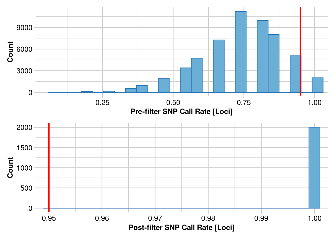
Completed: gl.filter.callrate
Starting gl.filter.callrate
  Processing genlight object with SNP data
  Warning: Data may include monomorphic loci in call rate
                    calculations for filtering
  Recalculating Call Rate
Removing loci based on Call Rate, threshold = 0.95 
Completed: gl.filter.callrate
Starting gl.filter.callrate
  Processing genlight object with SNP data
  Warning: Data may include monomorphic loci in call rate
                    calculations for filtering
  Recalculating Call Rate
Removing loci based on Call Rate, threshold = 0.95 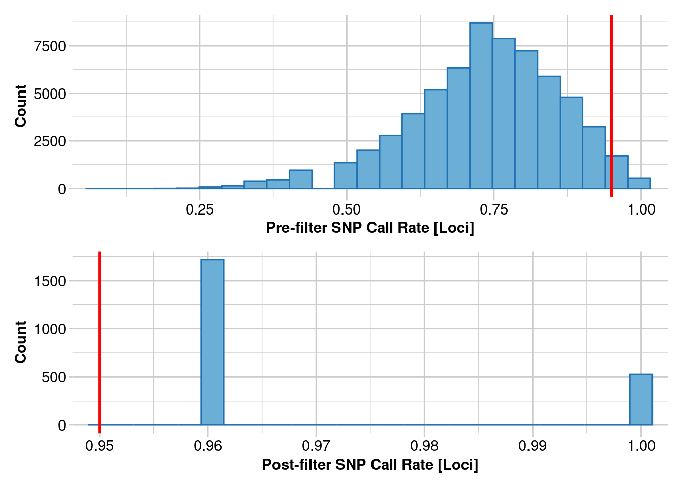
Completed: gl.filter.callrate
Starting gl.filter.callrate
  Processing genlight object with SNP data
  Warning: Data may include monomorphic loci in call rate
                    calculations for filtering
  Recalculating Call Rate
Removing loci based on Call Rate, threshold = 0.95 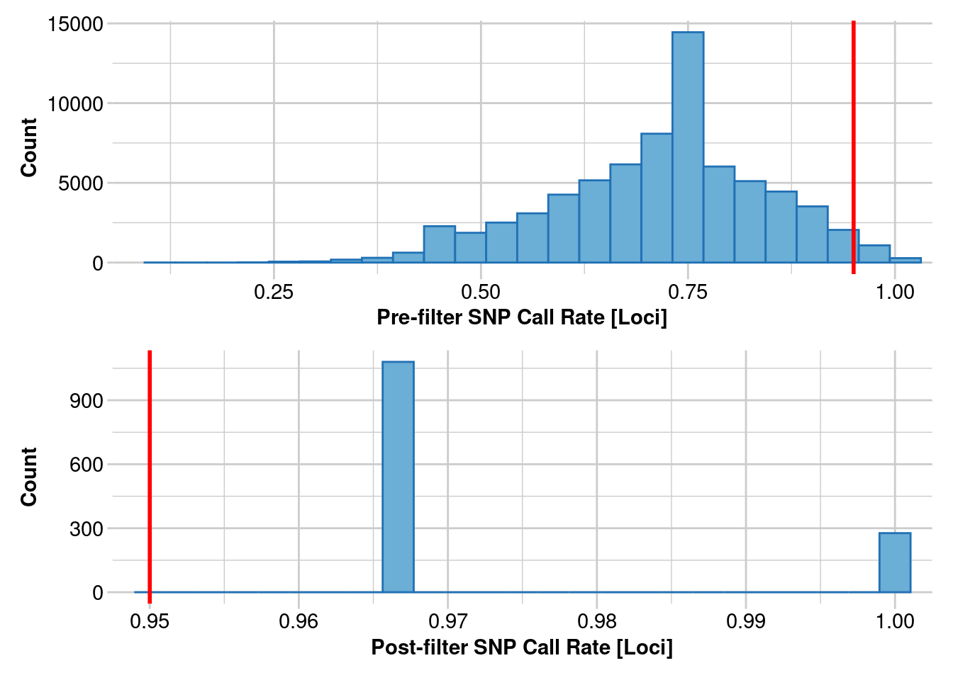
Completed: gl.filter.callrate
Starting gl.filter.callrate
  Processing genlight object with SNP data
  Warning: Data may include monomorphic loci in call rate
                    calculations for filtering
  Recalculating Call Rate
Removing loci based on Call Rate, threshold = 0.95 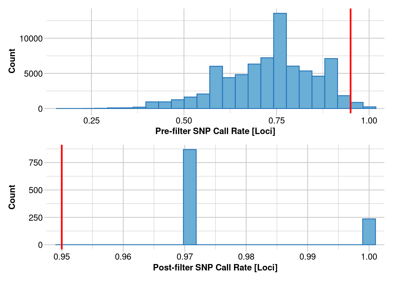
Completed: gl.filter.callrate
Starting gl.filter.callrate
  Processing genlight object with SNP data
  Warning: Data may include monomorphic loci in call rate
                    calculations for filtering
  Recalculating Call Rate
Removing loci based on Call Rate, threshold = 0.95 
Completed: gl.filter.callrate Calculate heterozygosity
# List all object names in the environment
all_names <- ls()

# Use grep() to match names that start with "Kimberley"
# and end with "0.95", .+ indicates any characters in between
kimberley_filtered <- grep("^Kimberley.+0\\.95$", all_names, value = TRUE)#put all the genlights into a mega list
#create another list with the ones we want
kimberley <- mget(kimberley_filtered)


#Initialize an empty data frame
heterozygosity_reports_df_0.95 <- data.frame()

# Iterate over the kimberley list to apply gl.report.heterozygosity
# and bind the results
for(name in names(kimberley)) {
  # Apply the function
  report <- gl.report.heterozygosity(kimberley[[name]])

  # Add 'ObjectName' as the first column of the report
  report <- cbind(ObjectName = name, report)

  # Bind this report to the main data frame
  heterozygosity_reports_df_0.95 <- bind_rows(heterozygosity_reports_df_0.95, report)
}
Starting gl.report.heterozygosity
Processing genlight object with SNP data
Calculating Observed Heterozygosities, averaged across
loci, for each population
Calculating Expected Heterozygosities
Starting gl.colors
Selected color type dis
Completed: gl.colors 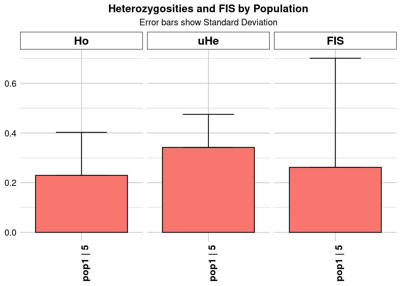
pop n.Ind n.Loc n.Loc.adj polyLoc monoLoc all_NALoc Ho HoSD
pop1 pop1 5 9335 1 9335 0 0 0.229502 0.173222
HoSE HoLCI HoHCI Ho.adj Ho.adjSD Ho.adjSE Ho.adjLCI Ho.adjHCI
pop1 0.001793 NA NA 0.229502 0.173222 0.001793 NA NA
He HeSD HeSE HeLCI HeHCI uHe uHeSD uHeSE uHeLCI
pop1 0.307878 0.119766 0.00124 NA NA 0.342087 0.133073 0.001377 NA
uHeHCI He.adj He.adjSD He.adjSE He.adjLCI He.adjHCI FIS FISSD
pop1 NA 0.307878 0.119766 0.00124 NA NA 0.261799 0.439324
FISSE FISLCI FISHCI
pop1 0.004547 NA NA
Completed: gl.report.heterozygosity
Starting gl.report.heterozygosity
  Processing genlight object with SNP data
  Calculating Observed Heterozygosities, averaged across
                    loci, for each population
  Calculating Expected Heterozygosities

Starting gl.colors
Selected color type dis
Completed: gl.colors 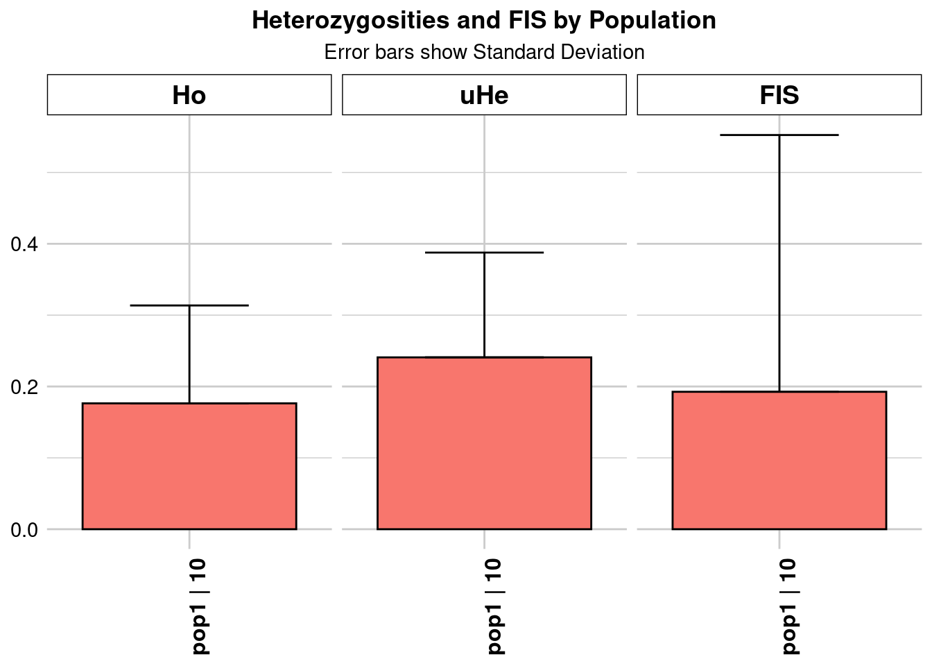
      pop n.Ind n.Loc n.Loc.adj polyLoc monoLoc all_NALoc       Ho     HoSD
pop1 pop1    10  5814         1    5814       0         0 0.176402 0.137187
         HoSE HoLCI HoHCI   Ho.adj Ho.adjSD Ho.adjSE Ho.adjLCI Ho.adjHCI
pop1 0.001799    NA    NA 0.176402 0.137187 0.001799        NA        NA
           He     HeSD    HeSE HeLCI HeHCI      uHe    uHeSD    uHeSE uHeLCI
pop1 0.228789 0.139511 0.00183    NA    NA 0.240831 0.146854 0.001926     NA
     uHeHCI   He.adj He.adjSD He.adjSE He.adjLCI He.adjHCI      FIS    FISSD
pop1     NA 0.228789 0.139511  0.00183        NA        NA 0.192591 0.359841
        FISSE FISLCI FISHCI
pop1 0.004719     NA     NA
Completed: gl.report.heterozygosity
Starting gl.report.heterozygosity
  Processing genlight object with SNP data
  Calculating Observed Heterozygosities, averaged across
                    loci, for each population
  Calculating Expected Heterozygosities

Starting gl.colors
Selected color type dis
Completed: gl.colors 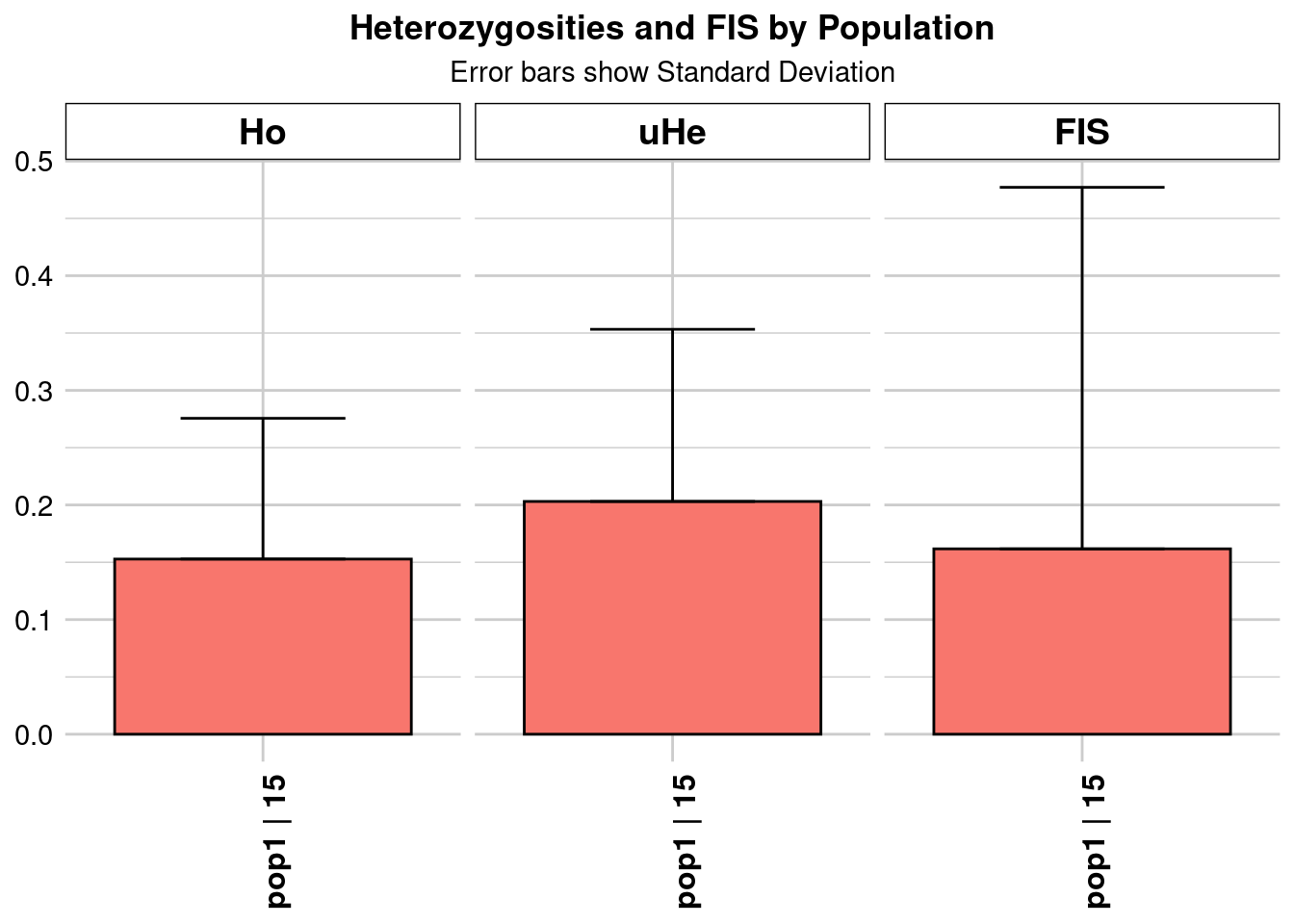
      pop n.Ind n.Loc n.Loc.adj polyLoc monoLoc all_NALoc       Ho     HoSD
pop1 pop1    15  2003         1    2003       0         0 0.152804 0.122813
         HoSE HoLCI HoHCI   Ho.adj Ho.adjSD Ho.adjSE Ho.adjLCI Ho.adjHCI
pop1 0.002744    NA    NA 0.152804 0.122813 0.002744        NA        NA
           He     HeSD     HeSE HeLCI HeHCI      uHe   uHeSD    uHeSE uHeLCI
pop1 0.196298 0.145174 0.003244    NA    NA 0.203067 0.15018 0.003356     NA
     uHeHCI   He.adj He.adjSD He.adjSE He.adjLCI He.adjHCI      FIS    FISSD
pop1     NA 0.196298 0.145174 0.003244        NA        NA 0.161721 0.315393
        FISSE FISLCI FISHCI
pop1 0.007047     NA     NA
Completed: gl.report.heterozygosity
Starting gl.report.heterozygosity
  Processing genlight object with SNP data
  Calculating Observed Heterozygosities, averaged across
                    loci, for each population
  Calculating Expected Heterozygosities

Starting gl.colors
Selected color type dis
Completed: gl.colors 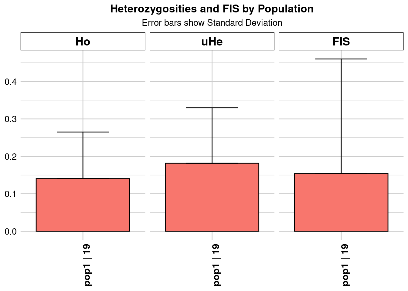
      pop    n.Ind n.Loc n.Loc.adj polyLoc monoLoc all_NALoc       Ho     HoSD
pop1 pop1 19.27864  4199         1    4199       0         0 0.140333 0.124561
         HoSE HoLCI HoHCI   Ho.adj Ho.adjSD Ho.adjSE Ho.adjLCI Ho.adjHCI
pop1 0.001922    NA    NA 0.140333 0.124561 0.001922        NA        NA
           He     HeSD     HeSE HeLCI HeHCI      uHe    uHeSD    uHeSE uHeLCI
pop1 0.177053 0.144114 0.002224    NA    NA 0.181767 0.147951 0.002283     NA
     uHeHCI   He.adj He.adjSD He.adjSE He.adjLCI He.adjHCI      FIS    FISSD
pop1     NA 0.177053 0.144114 0.002224        NA        NA 0.153933 0.306136
        FISSE FISLCI FISHCI
pop1 0.004724     NA     NA
Completed: gl.report.heterozygosity
Starting gl.report.heterozygosity
  Processing genlight object with SNP data
  Calculating Observed Heterozygosities, averaged across
                    loci, for each population
  Calculating Expected Heterozygosities

Starting gl.colors
Selected color type dis
Completed: gl.colors 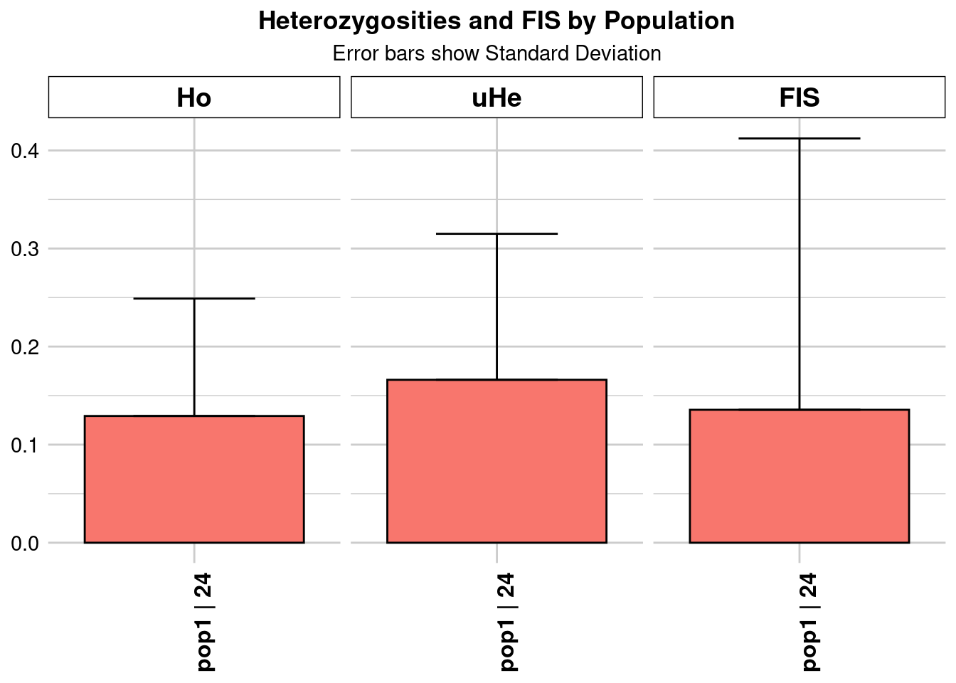
      pop   n.Ind n.Loc n.Loc.adj polyLoc monoLoc all_NALoc       Ho     HoSD
pop1 pop1 24.2354  2243         1    2243       0         0 0.129226 0.119719
         HoSE HoLCI HoHCI   Ho.adj Ho.adjSD Ho.adjSE Ho.adjLCI Ho.adjHCI
pop1 0.002528    NA    NA 0.129226 0.119719 0.002528        NA        NA
           He     HeSD     HeSE HeLCI HeHCI      uHe    uHeSD    uHeSE uHeLCI
pop1 0.162692 0.145793 0.003078    NA    NA 0.166119 0.148864 0.003143     NA
     uHeHCI   He.adj He.adjSD He.adjSE He.adjLCI He.adjHCI      FIS    FISSD
pop1     NA 0.162692 0.145793 0.003078        NA        NA 0.135561 0.276653
        FISSE FISLCI FISHCI
pop1 0.005841     NA     NA
Completed: gl.report.heterozygosity
Starting gl.report.heterozygosity
  Processing genlight object with SNP data
  Calculating Observed Heterozygosities, averaged across
                    loci, for each population
  Calculating Expected Heterozygosities

Starting gl.colors
Selected color type dis
Completed: gl.colors 
      pop    n.Ind n.Loc n.Loc.adj polyLoc monoLoc all_NALoc       Ho     HoSD
pop1 pop1 29.20428  1356         1    1356       0         0 0.117792 0.114525
        HoSE HoLCI HoHCI   Ho.adj Ho.adjSD Ho.adjSE Ho.adjLCI Ho.adjHCI
pop1 0.00311    NA    NA 0.117792 0.114525  0.00311        NA        NA
           He     HeSD     HeSE HeLCI HeHCI      uHe    uHeSD  uHeSE uHeLCI
pop1 0.147605 0.141139 0.003833    NA    NA 0.150176 0.143597 0.0039     NA
     uHeHCI   He.adj He.adjSD He.adjSE He.adjLCI He.adjHCI      FIS    FISSD
pop1     NA 0.147605 0.141139 0.003833        NA        NA 0.129329 0.267582
        FISSE FISLCI FISHCI
pop1 0.007267     NA     NA
Completed: gl.report.heterozygosity
Starting gl.report.heterozygosity
  Processing genlight object with SNP data
  Calculating Observed Heterozygosities, averaged across
                    loci, for each population
  Calculating Expected Heterozygosities

Starting gl.colors
Selected color type dis
Completed: gl.colors 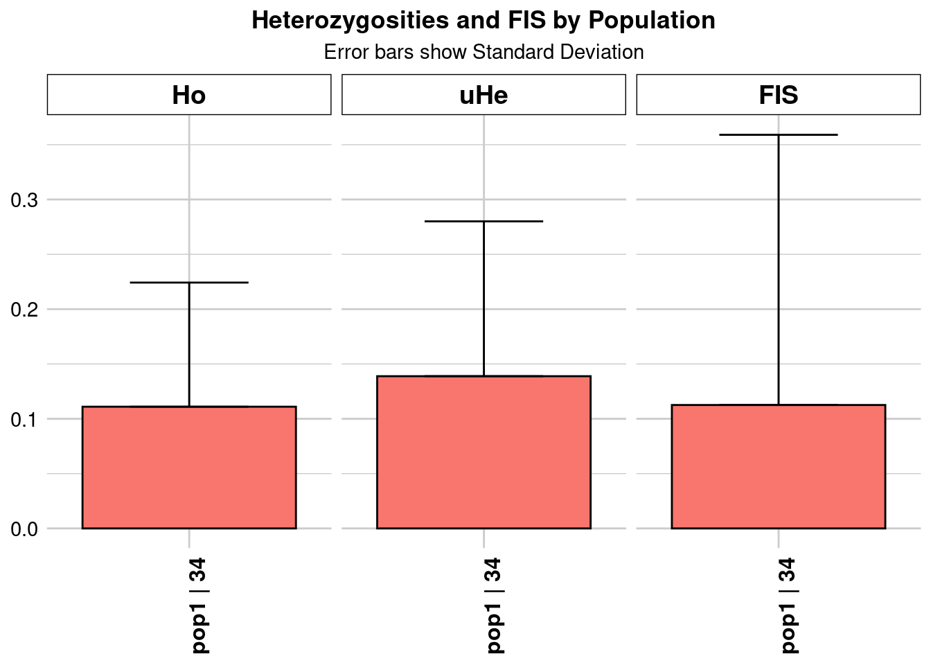
      pop    n.Ind n.Loc n.Loc.adj polyLoc monoLoc all_NALoc       Ho     HoSD
pop1 pop1 34.21357  1105         1    1105       0         0 0.111003 0.113222
         HoSE HoLCI HoHCI   Ho.adj Ho.adjSD Ho.adjSE Ho.adjLCI Ho.adjHCI
pop1 0.003406    NA    NA 0.111003 0.113222 0.003406        NA        NA
           He     HeSD     HeSE HeLCI HeHCI      uHe    uHeSD    uHeSE uHeLCI
pop1 0.136806 0.139159 0.004186    NA    NA 0.138835 0.141223 0.004248     NA
     uHeHCI   He.adj He.adjSD He.adjSE He.adjLCI He.adjHCI      FIS    FISSD
pop1     NA 0.136806 0.139159 0.004186        NA        NA 0.112563 0.246423
        FISSE FISLCI FISHCI
pop1 0.007413     NA     NA
Completed: gl.report.heterozygosity
Starting gl.report.heterozygosity
  Processing genlight object with SNP data
  Calculating Observed Heterozygosities, averaged across
                    loci, for each population
  Calculating Expected Heterozygosities

Starting gl.colors
Selected color type dis
Completed: gl.colors 
      pop    n.Ind n.Loc n.Loc.adj polyLoc monoLoc all_NALoc       Ho     HoSD
pop1 pop1 38.42546  1838         1    1838       0         0 0.110599 0.115467
         HoSE HoLCI HoHCI   Ho.adj Ho.adjSD Ho.adjSE Ho.adjLCI Ho.adjHCI
pop1 0.002693    NA    NA 0.110599 0.115467 0.002693        NA        NA
           He     HeSD     HeSE HeLCI HeHCI      uHe    uHeSD    uHeSE uHeLCI
pop1 0.137218 0.141699 0.003305    NA    NA 0.139027 0.143567 0.003349     NA
     uHeHCI   He.adj He.adjSD He.adjSE He.adjLCI He.adjHCI      FIS    FISSD
pop1     NA 0.137218 0.141699 0.003305        NA        NA 0.114931 0.246381
        FISSE FISLCI FISHCI
pop1 0.005747     NA     NA
Completed: gl.report.heterozygosity
# heterozygosity_reports_df now contains all the reports with an
# additional column for object names
knitr::kable(heterozygosity_reports_df_0.95)| ObjectName | pop | n.Ind | n.Loc | n.Loc.adj | polyLoc | monoLoc | all_NALoc | Ho | HoSD | HoSE | HoLCI | HoHCI | Ho.adj | Ho.adjSD | Ho.adjSE | Ho.adjLCI | Ho.adjHCI | He | HeSD | HeSE | HeLCI | HeHCI | uHe | uHeSD | uHeSE | uHeLCI | uHeHCI | He.adj | He.adjSD | He.adjSE | He.adjLCI | He.adjHCI | FIS | FISSD | FISSE | FISLCI | FISHCI | |
|---|---|---|---|---|---|---|---|---|---|---|---|---|---|---|---|---|---|---|---|---|---|---|---|---|---|---|---|---|---|---|---|---|---|---|---|---|---|---|
| pop1…1 | Kimberley_n_05.vcf_0.95 | pop1 | 5.00000 | 9335 | 1 | 9335 | 0 | 0 | 0.229502 | 0.173222 | 0.001793 | NA | NA | 0.229502 | 0.173222 | 0.001793 | NA | NA | 0.307878 | 0.119766 | 0.001240 | NA | NA | 0.342087 | 0.133073 | 0.001377 | NA | NA | 0.307878 | 0.119766 | 0.001240 | NA | NA | 0.261799 | 0.439324 | 0.004547 | NA | NA |
| pop1…2 | Kimberley_n_10.vcf_0.95 | pop1 | 10.00000 | 5814 | 1 | 5814 | 0 | 0 | 0.176402 | 0.137187 | 0.001799 | NA | NA | 0.176402 | 0.137187 | 0.001799 | NA | NA | 0.228789 | 0.139511 | 0.001830 | NA | NA | 0.240831 | 0.146854 | 0.001926 | NA | NA | 0.228789 | 0.139511 | 0.001830 | NA | NA | 0.192591 | 0.359841 | 0.004719 | NA | NA |
| pop1…3 | Kimberley_n_15.vcf_0.95 | pop1 | 15.00000 | 2003 | 1 | 2003 | 0 | 0 | 0.152804 | 0.122813 | 0.002744 | NA | NA | 0.152804 | 0.122813 | 0.002744 | NA | NA | 0.196298 | 0.145174 | 0.003244 | NA | NA | 0.203067 | 0.150180 | 0.003356 | NA | NA | 0.196298 | 0.145174 | 0.003244 | NA | NA | 0.161721 | 0.315393 | 0.007047 | NA | NA |
| pop1…4 | Kimberley_n_20.vcf_0.95 | pop1 | 19.27864 | 4199 | 1 | 4199 | 0 | 0 | 0.140333 | 0.124561 | 0.001922 | NA | NA | 0.140333 | 0.124561 | 0.001922 | NA | NA | 0.177053 | 0.144114 | 0.002224 | NA | NA | 0.181767 | 0.147951 | 0.002283 | NA | NA | 0.177053 | 0.144114 | 0.002224 | NA | NA | 0.153933 | 0.306136 | 0.004724 | NA | NA |
| pop1…5 | Kimberley_n_25.vcf_0.95 | pop1 | 24.23540 | 2243 | 1 | 2243 | 0 | 0 | 0.129226 | 0.119719 | 0.002528 | NA | NA | 0.129226 | 0.119719 | 0.002528 | NA | NA | 0.162692 | 0.145793 | 0.003078 | NA | NA | 0.166119 | 0.148864 | 0.003143 | NA | NA | 0.162692 | 0.145793 | 0.003078 | NA | NA | 0.135561 | 0.276653 | 0.005841 | NA | NA |
| pop1…6 | Kimberley_n_30.vcf_0.95 | pop1 | 29.20428 | 1356 | 1 | 1356 | 0 | 0 | 0.117792 | 0.114525 | 0.003110 | NA | NA | 0.117792 | 0.114525 | 0.003110 | NA | NA | 0.147605 | 0.141139 | 0.003833 | NA | NA | 0.150176 | 0.143597 | 0.003900 | NA | NA | 0.147605 | 0.141139 | 0.003833 | NA | NA | 0.129329 | 0.267582 | 0.007267 | NA | NA |
| pop1…7 | Kimberley_n_35.vcf_0.95 | pop1 | 34.21357 | 1105 | 1 | 1105 | 0 | 0 | 0.111003 | 0.113222 | 0.003406 | NA | NA | 0.111003 | 0.113222 | 0.003406 | NA | NA | 0.136806 | 0.139159 | 0.004186 | NA | NA | 0.138835 | 0.141223 | 0.004248 | NA | NA | 0.136806 | 0.139159 | 0.004186 | NA | NA | 0.112563 | 0.246423 | 0.007413 | NA | NA |
| pop1…8 | Kimberley_n_40.vcf_0.95 | pop1 | 38.42546 | 1838 | 1 | 1838 | 0 | 0 | 0.110599 | 0.115467 | 0.002693 | NA | NA | 0.110599 | 0.115467 | 0.002693 | NA | NA | 0.137218 | 0.141699 | 0.003305 | NA | NA | 0.139027 | 0.143567 | 0.003349 | NA | NA | 0.137218 | 0.141699 | 0.003305 | NA | NA | 0.114931 | 0.246381 | 0.005747 | NA | NA |
Plotting results
# Example using ggplot2 to plot the data
library(ggplot2)
kimberley_Ho_0.95callrate <- ggplot(heterozygosity_reports_df_0.95, aes(x = ObjectName, y = Ho)) +
  geom_point() +
  scale_y_continuous(limits = c(0, NA)) +
  theme(axis.text.x = element_text(angle = 65, hjust = 1)) +
  labs(title = "Observed Heterozygosity by Sample number 0.95 Call Rate",
       x = "Sample Number", y = "Observed Heterozygosity (Ho) at 0.95 Call Rate")
kimberley_Ho_0.95callrate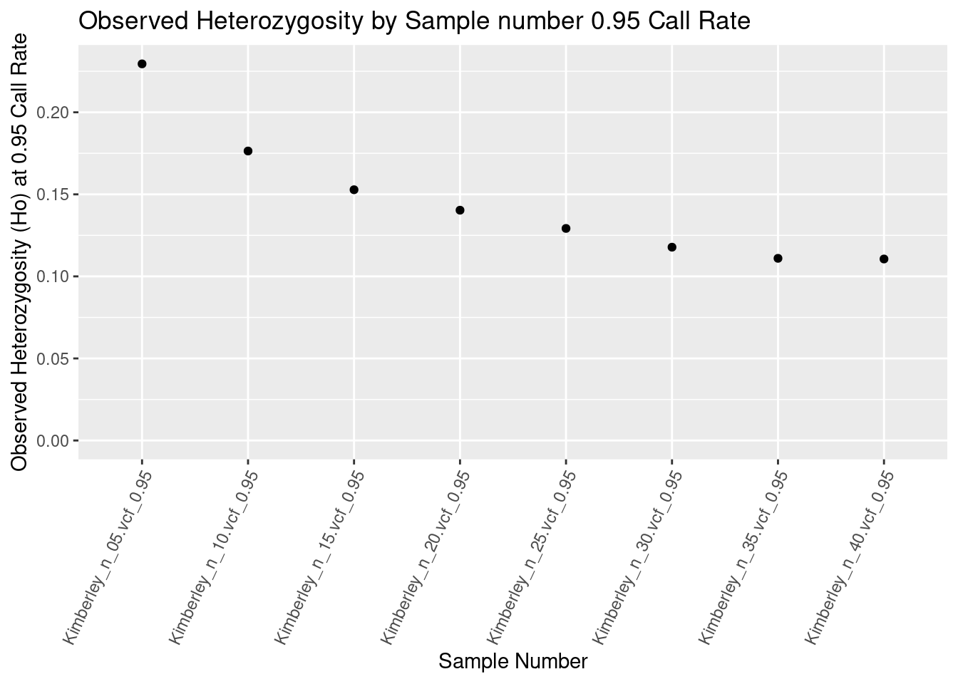
par(mfrow = c(2,1))
kimberley_Ho_0.7callrate +kimberley_Ho_0.95callrate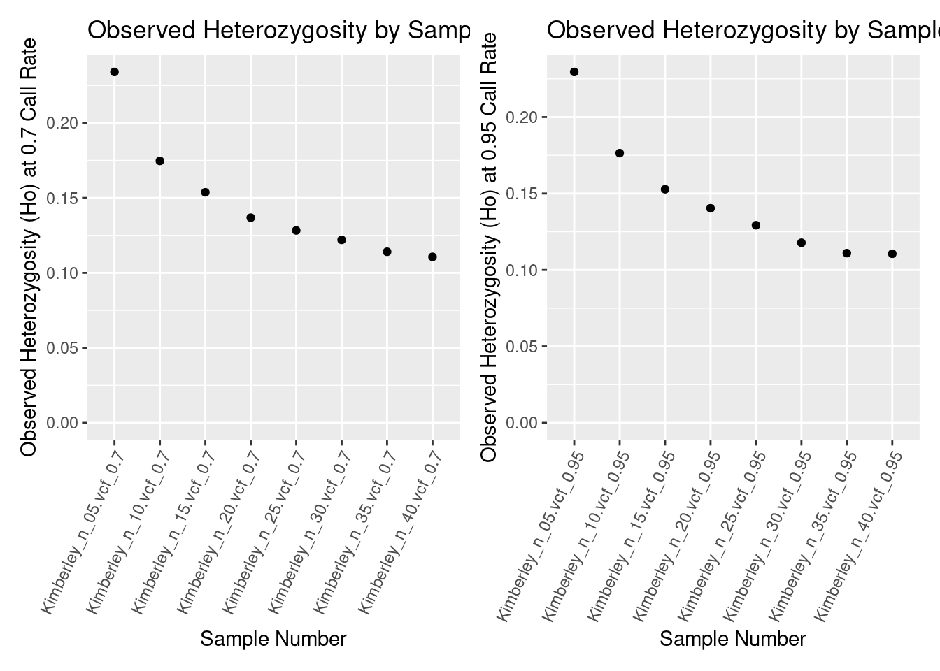
Call rate filters
Higher call rate filters can reduce your slightly reduce your heterozygosity estimate, but the major issue is sample number.
3. Estimating heterozygosity: Even sampling
does subsetting to have the same sample numbers fix the issue?
Let’s compare heterozygosity when SNPs are called on 5 individuals, versus called on 40 individuals and then subset to 5 individuals.
If you called SNPs on more individuals than you wanted to make them equal, can you just remove individuals without re-calling SNPS? Let’s test.
Subsampling
# Use grep() to match names that start with "Kimberley"
kimberley_names <- grep("^Kimberley.*\\.vcf$", all_names, value = TRUE)
# put all the genlights into a mega list

#create another list with the ones we want
kimberley <- mget(kimberley_names)

# Now lets subsample the datasets down to the same five individuals
# so that the only difference is our SNP calling
# who are the individuals
inds <- indNames(Kimberley_n_05.vcf_0.7)

#Initialize an empty data frame
heterozygosity_when_subsampling <- data.frame()

for(name in names(kimberley)) {
  # Access the genlight object from your list
  genlight_object <- kimberley[[name]]

  # Subset the individuals
  x <- gl.keep.ind(genlight_object, ind.list = inds, mono.rm = TRUE)

  #filter on call rate

  x <- gl.filter.callrate(x, threshold = .7)

  # Apply the function
  report <- gl.report.heterozygosity(x)

  # Add 'ObjectName' as the first column of the report
  report$ObjectName <- name
  # Adjusting to add column without cbind to maintain data frame classes

  # Bind this report to the main data frame
  heterozygosity_when_subsampling <- bind_rows(heterozygosity_when_subsampling,
                                               report)
}
Starting gl.keep.ind
Processing genlight object with SNP data
Warning: data include loci that are scored NA across all individuals.
Consider filtering using gl <- gl.filter.allna(gl)
Deleting all but the listed individuals Kimberley_ABTC102537_DLit20-5353_CE4Y2ANXX_1, Kimberley_ABTC11911_DLit20-5353_CE7VEANXX_1, Kimberley_ABTC86488_DLit20-5353_CECHMANXX_4, Kimberley_CCM7524_DLit20-5353_CECHMANXX_2, Kimberley_ABTC135731_DLit20-5353_CE7VEANXX_1
Deleting monomorphic loc
Locus metrics not recalculated
Completed: gl.keep.ind
Starting gl.filter.callrate
Processing genlight object with SNP data
Warning: Data may include monomorphic loci in call rate
calculations for filtering
Recalculating Call Rate
Removing loci based on Call Rate, threshold = 0.7 
Completed: gl.filter.callrate
Starting gl.report.heterozygosity
Processing genlight object with SNP data
Calculating Observed Heterozygosities, averaged across
loci, for each population
Calculating Expected Heterozygosities
Starting gl.colors
Selected color type dis
Completed: gl.colors 
pop n.Ind n.Loc n.Loc.adj polyLoc monoLoc all_NALoc Ho HoSD
pop1 pop1 4.327947 28465 1 28465 0 0 0.233986 0.190371
HoSE HoLCI HoHCI Ho.adj Ho.adjSD Ho.adjSE Ho.adjLCI Ho.adjHCI
pop1 0.001128 NA NA 0.233986 0.190371 0.001128 NA NA
He HeSD HeSE HeLCI HeHCI uHe uHeSD uHeSE uHeLCI
pop1 0.329375 0.112778 0.000668 NA NA 0.372398 0.127509 0.000756 NA
uHeHCI He.adj He.adjSD He.adjSE He.adjLCI He.adjHCI FIS FISSD
pop1 NA 0.329375 0.112778 0.000668 NA NA 0.302454 0.469498
FISSE FISLCI FISHCI
pop1 0.002783 NA NA
Completed: gl.report.heterozygosity
Starting gl.keep.ind
  Processing genlight object with SNP data
  Warning: data include loci that are scored NA across all individuals.
  Consider filtering using gl <- gl.filter.allna(gl)
  Deleting all but the listed individuals Kimberley_ABTC102537_DLit20-5353_CE4Y2ANXX_1, Kimberley_ABTC11911_DLit20-5353_CE7VEANXX_1, Kimberley_ABTC86488_DLit20-5353_CECHMANXX_4, Kimberley_CCM7524_DLit20-5353_CECHMANXX_2, Kimberley_ABTC135731_DLit20-5353_CE7VEANXX_1
  Deleting monomorphic loc
  Locus metrics not recalculated
Completed: gl.keep.ind
Starting gl.filter.callrate
  Processing genlight object with SNP data
  Warning: Data may include monomorphic loci in call rate
                    calculations for filtering
  Recalculating Call Rate
Removing loci based on Call Rate, threshold = 0.7 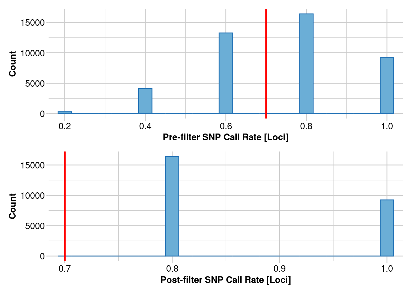
Completed: gl.filter.callrate
Starting gl.report.heterozygosity
  Processing genlight object with SNP data
  Calculating Observed Heterozygosities, averaged across
                    loci, for each population
  Calculating Expected Heterozygosities

Starting gl.colors
Selected color type dis
Completed: gl.colors 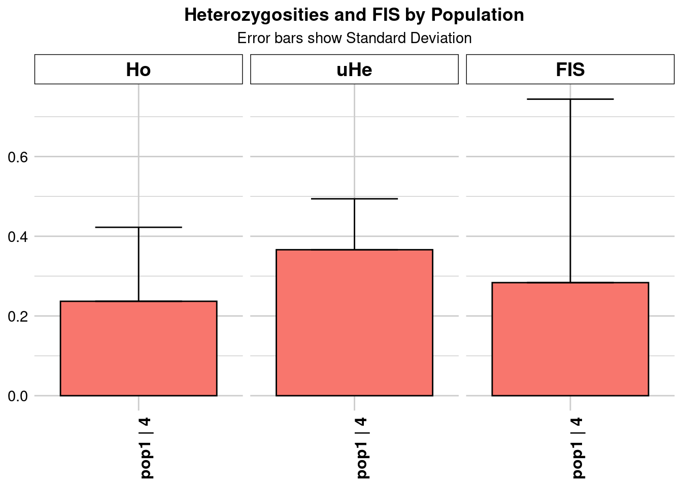
pop n.Ind n.Loc n.Loc.adj polyLoc monoLoc all_NALoc Ho HoSD
pop1 pop1 4.360384 25656 1 25656 0 0 0.236861 0.185631
HoSE HoLCI HoHCI Ho.adj Ho.adjSD Ho.adjSE Ho.adjLCI Ho.adjHCI
pop1 0.001159 NA NA 0.236861 0.185631 0.001159 NA NA
He HeSD HeSE HeLCI HeHCI uHe uHeSD uHeSE uHeLCI
pop1 0.324224 0.113105 0.000706 NA NA 0.366218 0.127754 0.000798 NA
uHeHCI He.adj He.adjSD He.adjSE He.adjLCI He.adjHCI FIS FISSD
pop1 NA 0.324224 0.113105 0.000706 NA NA 0.28369 0.460341
FISSE FISLCI FISHCI
pop1 0.002874 NA NA
Completed: gl.report.heterozygosity
Starting gl.keep.ind
Processing genlight object with SNP data
Deleting all but the listed individuals Kimberley_ABTC102537_DLit20-5353_CE4Y2ANXX_1, Kimberley_ABTC11911_DLit20-5353_CE7VEANXX_1, Kimberley_ABTC86488_DLit20-5353_CECHMANXX_4, Kimberley_CCM7524_DLit20-5353_CECHMANXX_2, Kimberley_ABTC135731_DLit20-5353_CE7VEANXX_1
Deleting monomorphic loc
Locus metrics not recalculated
Completed: gl.keep.ind
Starting gl.filter.callrate
Processing genlight object with SNP data
Warning: Data may include monomorphic loci in call rate
calculations for filtering
Recalculating Call Rate
Removing loci based on Call Rate, threshold = 0.7 
Completed: gl.filter.callrate
Starting gl.report.heterozygosity
  Processing genlight object with SNP data
  Calculating Observed Heterozygosities, averaged across
                    loci, for each population
  Calculating Expected Heterozygosities

Starting gl.colors
Selected color type dis
Completed: gl.colors 
pop n.Ind n.Loc n.Loc.adj polyLoc monoLoc all_NALoc Ho HoSD
pop1 pop1 4.404846 21171 1 21171 0 0 0.241755 0.181273
HoSE HoLCI HoHCI Ho.adj Ho.adjSD Ho.adjSE Ho.adjLCI Ho.adjHCI
pop1 0.001246 NA NA 0.241755 0.181273 0.001246 NA NA
He HeSD HeSE HeLCI HeHCI uHe uHeSD uHeSE uHeLCI
pop1 0.318786 0.113593 0.000781 NA NA 0.359605 0.128138 0.000881 NA
uHeHCI He.adj He.adjSD He.adjSE He.adjLCI He.adjHCI FIS FISSD
pop1 NA 0.318786 0.113593 0.000781 NA NA 0.259282 0.44866
FISSE FISLCI FISHCI
pop1 0.003084 NA NA
Completed: gl.report.heterozygosity
Starting gl.keep.ind
Processing genlight object with SNP data
Deleting all but the listed individuals Kimberley_ABTC102537_DLit20-5353_CE4Y2ANXX_1, Kimberley_ABTC11911_DLit20-5353_CE7VEANXX_1, Kimberley_ABTC86488_DLit20-5353_CECHMANXX_4, Kimberley_CCM7524_DLit20-5353_CECHMANXX_2, Kimberley_ABTC135731_DLit20-5353_CE7VEANXX_1
Deleting monomorphic loc
Locus metrics not recalculated
Completed: gl.keep.ind
Starting gl.filter.callrate
Processing genlight object with SNP data
Warning: Data may include monomorphic loci in call rate
calculations for filtering
Recalculating Call Rate
Removing loci based on Call Rate, threshold = 0.7 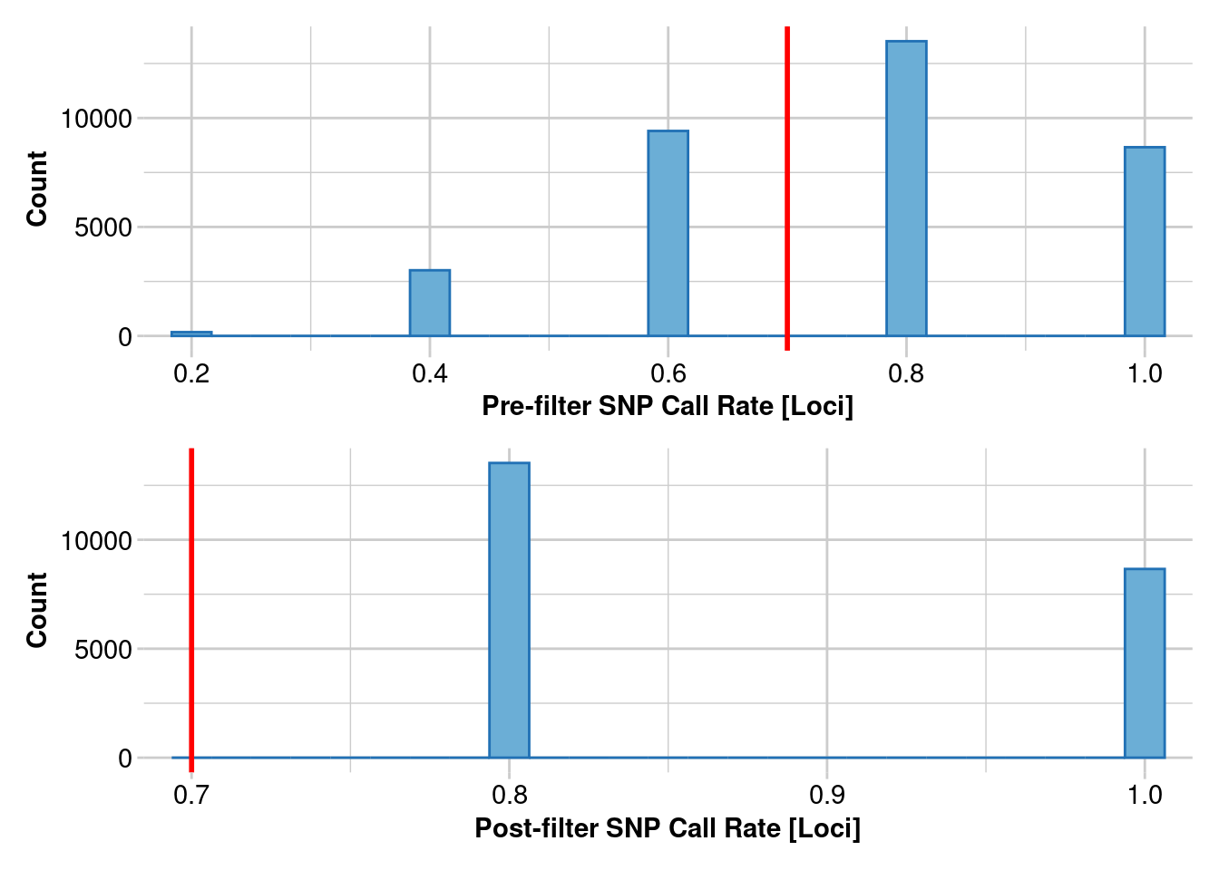
Completed: gl.filter.callrate
Starting gl.report.heterozygosity
  Processing genlight object with SNP data
  Calculating Observed Heterozygosities, averaged across
                    loci, for each population
  Calculating Expected Heterozygosities

Starting gl.colors
Selected color type dis
Completed: gl.colors 
pop n.Ind n.Loc n.Loc.adj polyLoc monoLoc all_NALoc Ho HoSD
pop1 pop1 4.390371 22184 1 22184 0 0 0.241731 0.181534
HoSE HoLCI HoHCI Ho.adj Ho.adjSD Ho.adjSE Ho.adjLCI Ho.adjHCI
pop1 0.001219 NA NA 0.241731 0.181534 0.001219 NA NA
He HeSD HeSE HeLCI HeHCI uHe uHeSD uHeSE uHeLCI
pop1 0.319324 0.113423 0.000762 NA NA 0.360365 0.128001 0.000859 NA
uHeHCI He.adj He.adjSD He.adjSE He.adjLCI He.adjHCI FIS FISSD
pop1 NA 0.319324 0.113423 0.000762 NA NA 0.260639 0.449285
FISSE FISLCI FISHCI
pop1 0.003016 NA NA
Completed: gl.report.heterozygosity
Starting gl.keep.ind
Processing genlight object with SNP data
Deleting all but the listed individuals Kimberley_ABTC102537_DLit20-5353_CE4Y2ANXX_1, Kimberley_ABTC11911_DLit20-5353_CE7VEANXX_1, Kimberley_ABTC86488_DLit20-5353_CECHMANXX_4, Kimberley_CCM7524_DLit20-5353_CECHMANXX_2, Kimberley_ABTC135731_DLit20-5353_CE7VEANXX_1
Deleting monomorphic loc
Locus metrics not recalculated
Completed: gl.keep.ind
Starting gl.filter.callrate
Processing genlight object with SNP data
Warning: Data may include monomorphic loci in call rate
calculations for filtering
Recalculating Call Rate
Removing loci based on Call Rate, threshold = 0.7 
Completed: gl.filter.callrate
Starting gl.report.heterozygosity
  Processing genlight object with SNP data
  Calculating Observed Heterozygosities, averaged across
                    loci, for each population
  Calculating Expected Heterozygosities

Starting gl.colors
Selected color type dis
Completed: gl.colors 
pop n.Ind n.Loc n.Loc.adj polyLoc monoLoc all_NALoc Ho HoSD
pop1 pop1 4.414982 19731 1 19731 0 0 0.243949 0.180217
HoSE HoLCI HoHCI Ho.adj Ho.adjSD Ho.adjSE Ho.adjLCI Ho.adjHCI
pop1 0.001283 NA NA 0.243949 0.180217 0.001283 NA NA
He HeSD HeSE HeLCI HeHCI uHe uHeSD uHeSE uHeLCI
pop1 0.317031 0.113598 0.000809 NA NA 0.35752 0.128106 0.000912 NA
uHeHCI He.adj He.adjSD He.adjSE He.adjLCI He.adjHCI FIS FISSD
pop1 NA 0.317031 0.113598 0.000809 NA NA 0.250234 0.444447
FISSE FISLCI FISHCI
pop1 0.003164 NA NA
Completed: gl.report.heterozygosity
Starting gl.keep.ind
Processing genlight object with SNP data
Deleting all but the listed individuals Kimberley_ABTC102537_DLit20-5353_CE4Y2ANXX_1, Kimberley_ABTC11911_DLit20-5353_CE7VEANXX_1, Kimberley_ABTC86488_DLit20-5353_CECHMANXX_4, Kimberley_CCM7524_DLit20-5353_CECHMANXX_2, Kimberley_ABTC135731_DLit20-5353_CE7VEANXX_1
Deleting monomorphic loc
Locus metrics not recalculated
Completed: gl.keep.ind
Starting gl.filter.callrate
Processing genlight object with SNP data
Warning: Data may include monomorphic loci in call rate
calculations for filtering
Recalculating Call Rate
Removing loci based on Call Rate, threshold = 0.7 
Completed: gl.filter.callrate
Starting gl.report.heterozygosity
  Processing genlight object with SNP data
  Calculating Observed Heterozygosities, averaged across
                    loci, for each population
  Calculating Expected Heterozygosities

Starting gl.colors
Selected color type dis
Completed: gl.colors 
pop n.Ind n.Loc n.Loc.adj polyLoc monoLoc all_NALoc Ho HoSD
pop1 pop1 4.404714 20239 1 20239 0 0 0.242991 0.179167
HoSE HoLCI HoHCI Ho.adj Ho.adjSD Ho.adjSE Ho.adjLCI Ho.adjHCI
pop1 0.001259 NA NA 0.242991 0.179167 0.001259 NA NA
He HeSD HeSE HeLCI HeHCI uHe uHeSD uHeSE uHeLCI
pop1 0.316909 0.113413 0.000797 NA NA 0.35749 0.127936 0.000899 NA
uHeHCI He.adj He.adjSD He.adjSE He.adjLCI He.adjHCI FIS FISSD
pop1 NA 0.316909 0.113413 0.000797 NA NA 0.251896 0.444278
FISSE FISLCI FISHCI
pop1 0.003123 NA NA
Completed: gl.report.heterozygosity
Starting gl.keep.ind
Processing genlight object with SNP data
Deleting all but the listed individuals Kimberley_ABTC102537_DLit20-5353_CE4Y2ANXX_1, Kimberley_ABTC11911_DLit20-5353_CE7VEANXX_1, Kimberley_ABTC86488_DLit20-5353_CECHMANXX_4, Kimberley_CCM7524_DLit20-5353_CECHMANXX_2, Kimberley_ABTC135731_DLit20-5353_CE7VEANXX_1
Deleting monomorphic loc
Locus metrics not recalculated
Completed: gl.keep.ind
Starting gl.filter.callrate
Processing genlight object with SNP data
Warning: Data may include monomorphic loci in call rate
calculations for filtering
Recalculating Call Rate
Removing loci based on Call Rate, threshold = 0.7 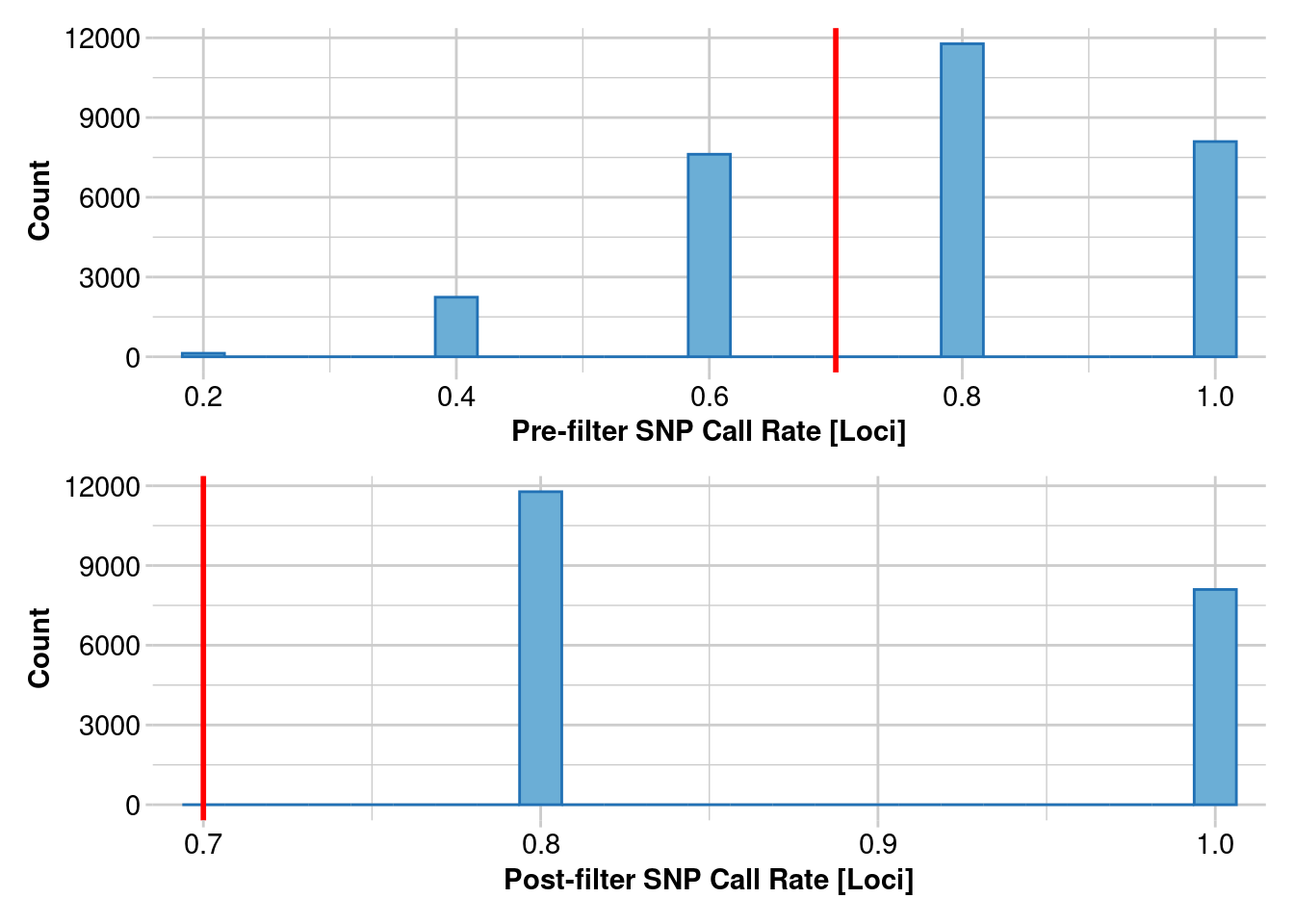
Completed: gl.filter.callrate
Starting gl.report.heterozygosity
  Processing genlight object with SNP data
  Calculating Observed Heterozygosities, averaged across
                    loci, for each population
  Calculating Expected Heterozygosities

Starting gl.colors
Selected color type dis
Completed: gl.colors 
pop n.Ind n.Loc n.Loc.adj polyLoc monoLoc all_NALoc Ho HoSD
pop1 pop1 4.407437 19873 1 19873 0 0 0.244377 0.179303
HoSE HoLCI HoHCI Ho.adj Ho.adjSD Ho.adjSE Ho.adjLCI Ho.adjHCI
pop1 0.001272 NA NA 0.244377 0.179303 0.001272 NA NA
He HeSD HeSE HeLCI HeHCI uHe uHeSD uHeSE uHeLCI
pop1 0.316308 0.113527 0.000805 NA NA 0.356783 0.128054 0.000908 NA
uHeHCI He.adj He.adjSD He.adjSE He.adjLCI He.adjHCI FIS FISSD
pop1 NA 0.316308 0.113527 0.000805 NA NA 0.247269 0.44271
FISSE FISLCI FISHCI
pop1 0.00314 NA NA
Completed: gl.report.heterozygosity
Starting gl.keep.ind
Processing genlight object with SNP data
Deleting all but the listed individuals Kimberley_ABTC102537_DLit20-5353_CE4Y2ANXX_1, Kimberley_ABTC11911_DLit20-5353_CE7VEANXX_1, Kimberley_ABTC86488_DLit20-5353_CECHMANXX_4, Kimberley_CCM7524_DLit20-5353_CECHMANXX_2, Kimberley_ABTC135731_DLit20-5353_CE7VEANXX_1
Deleting monomorphic loc
Locus metrics not recalculated
Completed: gl.keep.ind
Starting gl.filter.callrate
Processing genlight object with SNP data
Warning: Data may include monomorphic loci in call rate
calculations for filtering
Recalculating Call Rate
Removing loci based on Call Rate, threshold = 0.7 
Completed: gl.filter.callrate
Starting gl.report.heterozygosity
  Processing genlight object with SNP data
  Calculating Observed Heterozygosities, averaged across
                    loci, for each population
  Calculating Expected Heterozygosities

Starting gl.colors
Selected color type dis
Completed: gl.colors 
pop n.Ind n.Loc n.Loc.adj polyLoc monoLoc all_NALoc Ho HoSD
pop1 pop1 4.404922 20073 1 20073 0 0 0.244488 0.179823
HoSE HoLCI HoHCI Ho.adj Ho.adjSD Ho.adjSE Ho.adjLCI Ho.adjHCI
pop1 0.001269 NA NA 0.244488 0.179823 0.001269 NA NA
He HeSD HeSE HeLCI HeHCI uHe uHeSD uHeSE uHeLCI
pop1 0.316304 0.113509 0.000801 NA NA 0.356805 0.128043 0.000904 NA
uHeHCI He.adj He.adjSD He.adjSE He.adjLCI He.adjHCI FIS FISSD
pop1 NA 0.316304 0.113509 0.000801 NA NA 0.247144 0.443154
FISSE FISLCI FISHCI
pop1 0.003128 NA NA
Completed: gl.report.heterozygosity Plotting results
kimberley_Ho_subsampling <- ggplot(heterozygosity_when_subsampling, aes(x = ObjectName, y = Ho)) +
geom_point() +
scale_y_continuous(limits = c(0, NA)) +
theme(axis.text.x = element_text(angle = 65, hjust = 1)) +
labs(title = "Observed Heterozygosity when subsampling",
x = "SNP Calling", y = "Observed Heterozygosity (Ho)")
kimberley_Ho_subsampling
subsampling
There are some minor differences but it’s not too bad so this may be okay in some circumstances.
Subsampling more populations
There appears to be minor differences between sample sizes for the Kimberley population, but is this true for all populations?
Southeast
#create a list of the southeast genlights
Southeast_names <- ls(pattern = "^SouthEast")
#put all the genlights into a mega list
southeast <- mget(Southeast_names)
#Now lets subsample the datasets down to the same five individuals
#so that the only difference is our SNP calling
#who are the individuals
inds <- indNames(SouthEast_n_05.vcf)
for(name in names(southeast)) {
# Access the genlight object from your list
genlight_object <- southeast[[name]]
# Subset the individuals
x <- gl.keep.ind(genlight_object, ind.list = inds, mono.rm = TRUE)
#filter on call rate
x <- gl.filter.callrate(x, threshold = .7)
# Apply the function
report <- gl.report.heterozygosity(x)
# Add 'ObjectName' as the first column of the report
report$ObjectName <- name # Adjusting to add column without cbind to maintain data frame classes
# Bind this report to the main data frame
heterozygosity_when_subsampling <- bind_rows(heterozygosity_when_subsampling, report)
}Starting gl.keep.ind
Processing genlight object with SNP data
Warning: data include loci that are scored NA across all individuals.
Consider filtering using gl <- gl.filter.allna(gl)
Deleting all but the listed individuals SouthEast_ABTC92145_DLit20-5353_CECHMANXX_3, SouthEast_ABTC112638_DLit20-5353_CE7VEANXX_1, SouthEast_AMR164735_DLit20-5353_CE7VEANXX_1, SouthEast_ABTC38934_DLit20-5353_CECHMANXX_3, SouthEast_ABTC111142_DLit20-5353_CECHMANXX_3
Deleting monomorphic loc
Locus metrics not recalculated
Completed: gl.keep.ind
Starting gl.filter.callrate
Processing genlight object with SNP data
Warning: Data may include monomorphic loci in call rate
calculations for filtering
Recalculating Call Rate
Removing loci based on Call Rate, threshold = 0.7 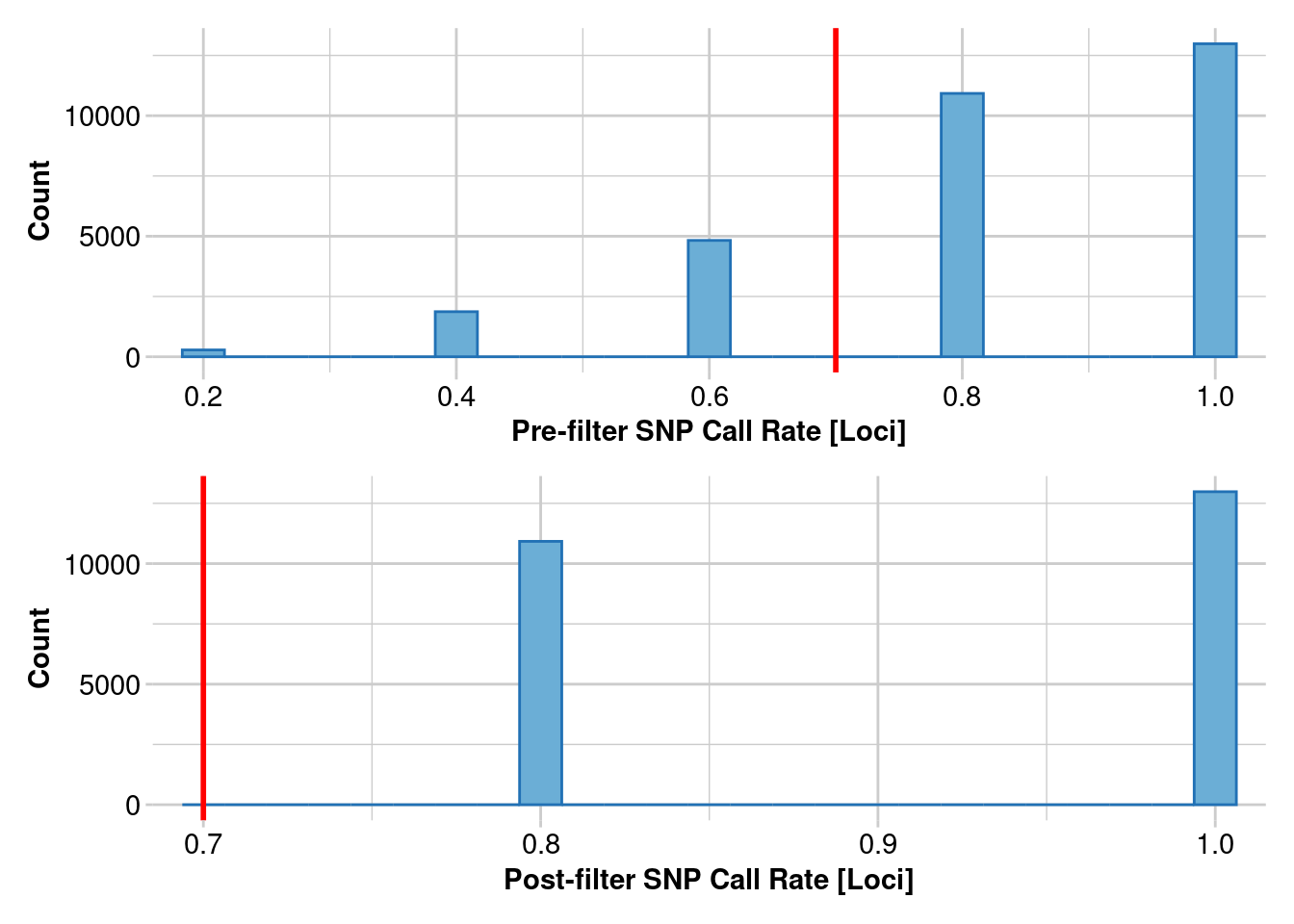
Completed: gl.filter.callrate
Starting gl.report.heterozygosity
  Processing genlight object with SNP data
  Calculating Observed Heterozygosities, averaged across
                    loci, for each population
  Calculating Expected Heterozygosities

Starting gl.colors
Selected color type dis
Completed: gl.colors 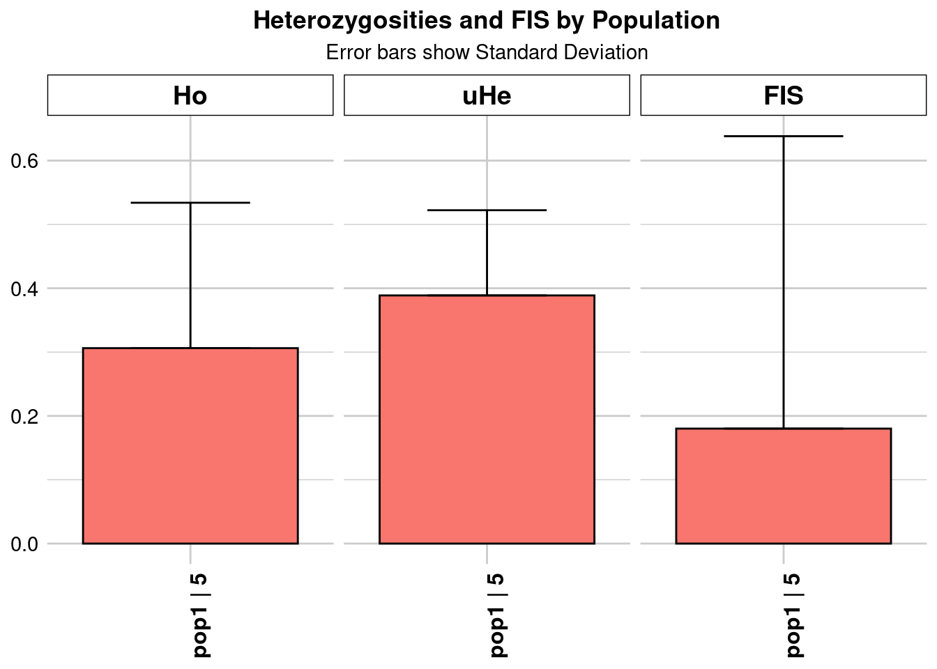
pop n.Ind n.Loc n.Loc.adj polyLoc monoLoc all_NALoc Ho HoSD
pop1 pop1 4.543063 23907 1 23907 0 0 0.306134 0.227794
HoSE HoLCI HoHCI Ho.adj Ho.adjSD Ho.adjSE Ho.adjLCI Ho.adjHCI
pop1 0.001473 NA NA 0.306134 0.227794 0.001473 NA NA
He HeSD HeSE HeLCI HeHCI uHe uHeSD uHeSE uHeLCI
pop1 0.345947 0.118783 0.000768 NA NA 0.38873 0.133473 0.000863 NA
uHeHCI He.adj He.adjSD He.adjSE He.adjLCI He.adjHCI FIS FISSD
pop1 NA 0.345947 0.118783 0.000768 NA NA 0.18011 0.458069
FISSE FISLCI FISHCI
pop1 0.002963 NA NA
Completed: gl.report.heterozygosity
Starting gl.keep.ind
  Processing genlight object with SNP data
  Warning: data include loci that are scored NA across all individuals.
  Consider filtering using gl <- gl.filter.allna(gl)
  Deleting all but the listed individuals SouthEast_ABTC92145_DLit20-5353_CECHMANXX_3, SouthEast_ABTC112638_DLit20-5353_CE7VEANXX_1, SouthEast_AMR164735_DLit20-5353_CE7VEANXX_1, SouthEast_ABTC38934_DLit20-5353_CECHMANXX_3, SouthEast_ABTC111142_DLit20-5353_CECHMANXX_3
  Deleting monomorphic loc
  Locus metrics not recalculated
Completed: gl.keep.ind
Starting gl.filter.callrate
  Processing genlight object with SNP data
  Warning: Data may include monomorphic loci in call rate
                    calculations for filtering
  Recalculating Call Rate
Removing loci based on Call Rate, threshold = 0.7 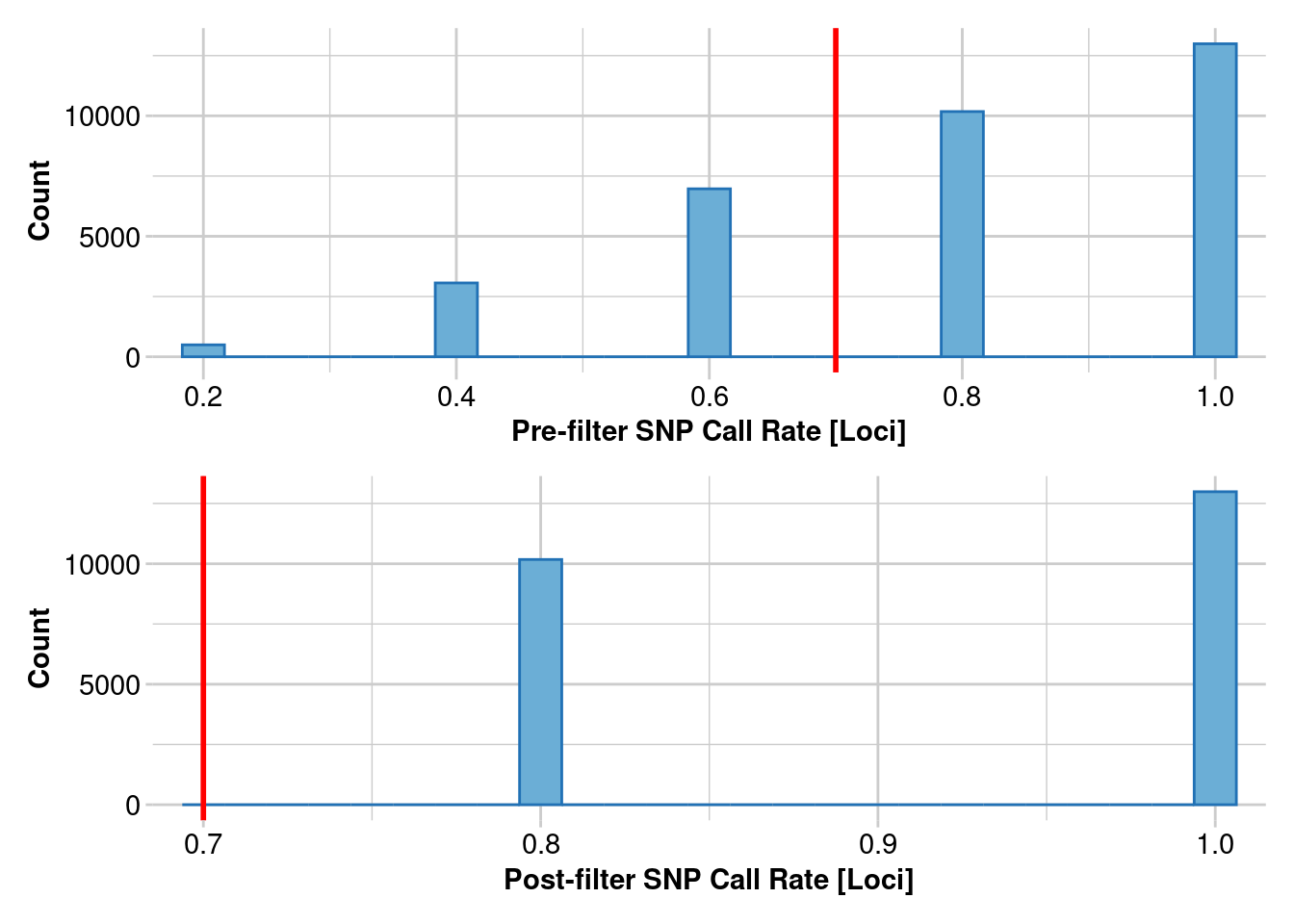
Completed: gl.filter.callrate
Starting gl.report.heterozygosity
  Processing genlight object with SNP data
  Calculating Observed Heterozygosities, averaged across
                    loci, for each population
  Calculating Expected Heterozygosities

Starting gl.colors
Selected color type dis
Completed: gl.colors 
pop n.Ind n.Loc n.Loc.adj polyLoc monoLoc all_NALoc Ho HoSD
pop1 pop1 4.560711 23167 1 23167 0 0 0.30276 0.21977
HoSE HoLCI HoHCI Ho.adj Ho.adjSD Ho.adjSE Ho.adjLCI Ho.adjHCI
pop1 0.001444 NA NA 0.30276 0.21977 0.001444 NA NA
He HeSD HeSE HeLCI HeHCI uHe uHeSD uHeSE uHeLCI
pop1 0.340234 0.119545 0.000785 NA NA 0.382127 0.134265 0.000882 NA
uHeHCI He.adj He.adjSD He.adjSE He.adjLCI He.adjHCI FIS FISSD
pop1 NA 0.340234 0.119545 0.000785 NA NA 0.172587 0.445217
FISSE FISLCI FISHCI
pop1 0.002925 NA NA
Completed: gl.report.heterozygosity
Starting gl.keep.ind
Processing genlight object with SNP data
Warning: data include loci that are scored NA across all individuals.
Consider filtering using gl <- gl.filter.allna(gl)
Deleting all but the listed individuals SouthEast_ABTC92145_DLit20-5353_CECHMANXX_3, SouthEast_ABTC112638_DLit20-5353_CE7VEANXX_1, SouthEast_AMR164735_DLit20-5353_CE7VEANXX_1, SouthEast_ABTC38934_DLit20-5353_CECHMANXX_3, SouthEast_ABTC111142_DLit20-5353_CECHMANXX_3
Deleting monomorphic loc
Locus metrics not recalculated
Completed: gl.keep.ind
Starting gl.filter.callrate
Processing genlight object with SNP data
Warning: Data may include monomorphic loci in call rate
calculations for filtering
Recalculating Call Rate
Removing loci based on Call Rate, threshold = 0.7 
Completed: gl.filter.callrate
Starting gl.report.heterozygosity
  Processing genlight object with SNP data
  Calculating Observed Heterozygosities, averaged across
                    loci, for each population
  Calculating Expected Heterozygosities

Starting gl.colors
Selected color type dis
Completed: gl.colors 
pop n.Ind n.Loc n.Loc.adj polyLoc monoLoc all_NALoc Ho HoSD
pop1 pop1 4.584442 21956 1 21956 0 0 0.300644 0.212385
HoSE HoLCI HoHCI Ho.adj Ho.adjSD Ho.adjSE Ho.adjLCI Ho.adjHCI
pop1 0.001433 NA NA 0.300644 0.212385 0.001433 NA NA
He HeSD HeSE HeLCI HeHCI uHe uHeSD uHeSE uHeLCI
pop1 0.337159 0.119975 0.00081 NA NA 0.378432 0.134662 0.000909 NA
uHeHCI He.adj He.adjSD He.adjSE He.adjLCI He.adjHCI FIS FISSD
pop1 NA 0.337159 0.119975 0.00081 NA NA 0.168427 0.433861
FISSE FISLCI FISHCI
pop1 0.002928 NA NA
Completed: gl.report.heterozygosity
Starting gl.keep.ind
Processing genlight object with SNP data
Deleting all but the listed individuals SouthEast_ABTC92145_DLit20-5353_CECHMANXX_3, SouthEast_ABTC112638_DLit20-5353_CE7VEANXX_1, SouthEast_AMR164735_DLit20-5353_CE7VEANXX_1, SouthEast_ABTC38934_DLit20-5353_CECHMANXX_3, SouthEast_ABTC111142_DLit20-5353_CECHMANXX_3
Deleting monomorphic loc
Locus metrics not recalculated
Completed: gl.keep.ind
Starting gl.filter.callrate
Processing genlight object with SNP data
Warning: Data may include monomorphic loci in call rate
calculations for filtering
Recalculating Call Rate
Removing loci based on Call Rate, threshold = 0.7 
Completed: gl.filter.callrate
Starting gl.report.heterozygosity
  Processing genlight object with SNP data
  Calculating Observed Heterozygosities, averaged across
                    loci, for each population
  Calculating Expected Heterozygosities

Starting gl.colors
Selected color type dis
Completed: gl.colors 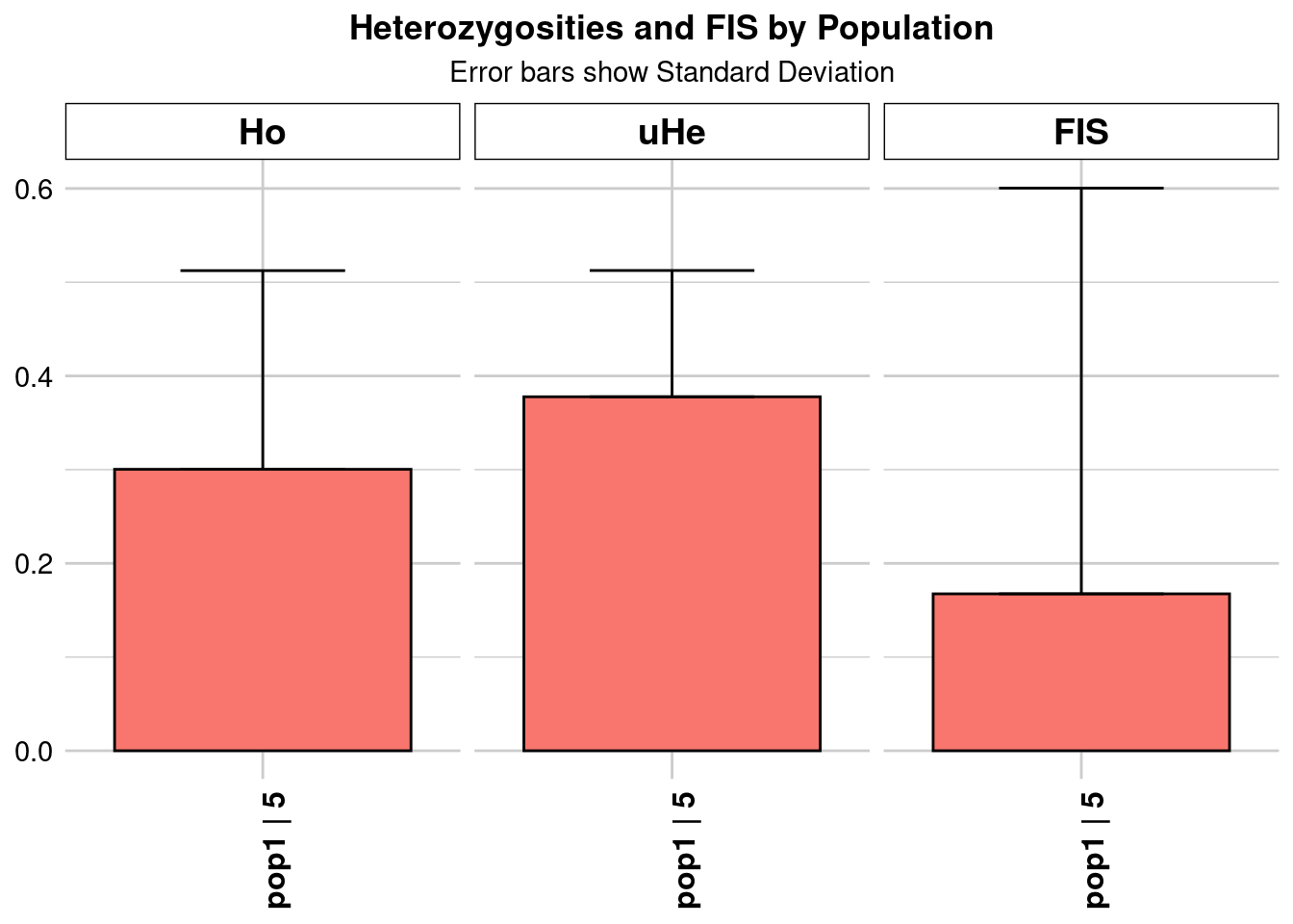
pop n.Ind n.Loc n.Loc.adj polyLoc monoLoc all_NALoc Ho HoSD
pop1 pop1 4.575179 22513 1 22513 0 0 0.300346 0.212014
HoSE HoLCI HoHCI Ho.adj Ho.adjSD Ho.adjSE Ho.adjLCI Ho.adjHCI
pop1 0.001413 NA NA 0.300346 0.212014 0.001413 NA NA
He HeSD HeSE HeLCI HeHCI uHe uHeSD uHeSE uHeLCI
pop1 0.336459 0.120052 8e-04 NA NA 0.37774 0.134782 0.000898 NA
uHeHCI He.adj He.adjSD He.adjSE He.adjLCI He.adjHCI FIS FISSD
pop1 NA 0.336459 0.120052 8e-04 NA NA 0.167435 0.432974
FISSE FISLCI FISHCI
pop1 0.002886 NA NA
Completed: gl.report.heterozygosity southeast_Ho_subsampling <- ggplot(heterozygosity_when_subsampling, aes(x = ObjectName, y = Ho)) +
geom_point() +
scale_y_continuous(limits = c(0, NA)) +
theme(axis.text.x = element_text(angle = 65, hjust = 1)) +
labs(title = "Observed Heterozygosity when subsampling",
x = "SNP Calling", y = "Observed Heterozygosity (Ho)")Central
#create a list of the central australian genlights
central_names <- ls(pattern = "^Central")
#put all the genlights into a mega list
central <- mget(central_names)
#Now lets subsample the datasets down to the same five individuals
#so that the only difference is our SNP calling
#who are the individuals
inds <- indNames(Central_n_05.vcf)
for(name in names(central)) {
# Access the genlight object from your list
genlight_object <- central[[name]]
# Subset the individuals
x <- gl.keep.ind(genlight_object, ind.list = inds, mono.rm = TRUE)
#filter on call rate
x <- gl.filter.callrate(x, threshold = .7)
# Apply the function
report <- gl.report.heterozygosity(x)
# Add 'ObjectName' as the first column of the report
report$ObjectName <- name # Adjusting to add column without cbind to maintain data frame classes
# Bind this report to the main data frame
heterozygosity_when_subsampling <- bind_rows(heterozygosity_when_subsampling, report)
}Starting gl.keep.ind
Processing genlight object with SNP data
Warning: data include loci that are scored NA across all individuals.
Consider filtering using gl <- gl.filter.allna(gl)
Deleting all but the listed individuals Central_ABTC12035_DLit20-5353_CECHMANXX_3, Central_ABTC36027_DLit20-5353_CECHMANXX_4, Central_ABTC9964_DLit20-5353_CE4Y2ANXX_5, Central_ABTC30246_DLit20-5353_CECHMANXX_3, Central_ABTC58795_DLit20-5353_CE4Y2ANXX_5
Deleting monomorphic loc
Locus metrics not recalculated
Completed: gl.keep.ind
Starting gl.filter.callrate
Processing genlight object with SNP data
Warning: Data may include monomorphic loci in call rate
calculations for filtering
Recalculating Call Rate
Removing loci based on Call Rate, threshold = 0.7 
Completed: gl.filter.callrate
Starting gl.report.heterozygosity
  Processing genlight object with SNP data
  Calculating Observed Heterozygosities, averaged across
                    loci, for each population
  Calculating Expected Heterozygosities

Starting gl.colors
Selected color type dis
Completed: gl.colors 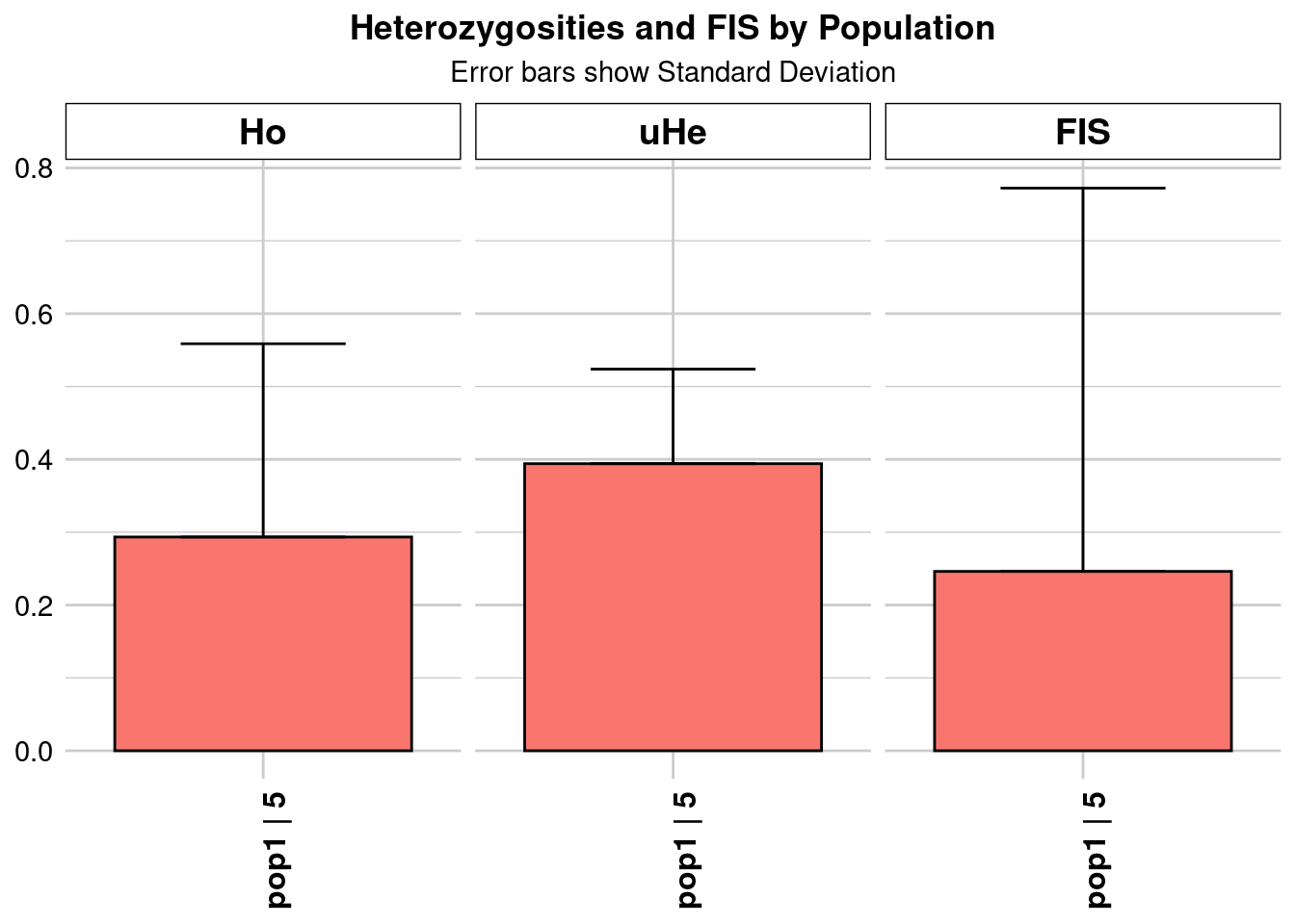
pop n.Ind n.Loc n.Loc.adj polyLoc monoLoc all_NALoc Ho HoSD
pop1 pop1 4.591516 20745 1 20745 0 0 0.293408 0.265273
HoSE HoLCI HoHCI Ho.adj Ho.adjSD Ho.adjSE Ho.adjLCI Ho.adjHCI
pop1 0.001842 NA NA 0.293408 0.265273 0.001842 NA NA
He HeSD HeSE HeLCI HeHCI uHe uHeSD uHeSE uHeLCI
pop1 0.35118 0.115651 0.000803 NA NA 0.394095 0.129784 0.000901 NA
uHeHCI He.adj He.adjSD He.adjSE He.adjLCI He.adjHCI FIS FISSD
pop1 NA 0.35118 0.115651 0.000803 NA NA 0.246186 0.526134
FISSE FISLCI FISHCI
pop1 0.003653 NA NA
Completed: gl.report.heterozygosity
Starting gl.keep.ind
  Processing genlight object with SNP data
  Warning: data include loci that are scored NA across all individuals.
  Consider filtering using gl <- gl.filter.allna(gl)
  Deleting all but the listed individuals Central_ABTC12035_DLit20-5353_CECHMANXX_3, Central_ABTC36027_DLit20-5353_CECHMANXX_4, Central_ABTC9964_DLit20-5353_CE4Y2ANXX_5, Central_ABTC30246_DLit20-5353_CECHMANXX_3, Central_ABTC58795_DLit20-5353_CE4Y2ANXX_5
  Deleting monomorphic loc
  Locus metrics not recalculated
Completed: gl.keep.ind
Starting gl.filter.callrate
  Processing genlight object with SNP data
  Warning: Data may include monomorphic loci in call rate
                    calculations for filtering
  Recalculating Call Rate
Removing loci based on Call Rate, threshold = 0.7 
Completed: gl.filter.callrate
Starting gl.report.heterozygosity
  Processing genlight object with SNP data
  Calculating Observed Heterozygosities, averaged across
                    loci, for each population
  Calculating Expected Heterozygosities

Starting gl.colors
Selected color type dis
Completed: gl.colors 
pop n.Ind n.Loc n.Loc.adj polyLoc monoLoc all_NALoc Ho HoSD
pop1 pop1 4.612141 20064 1 20064 0 0 0.281935 0.253619
HoSE HoLCI HoHCI Ho.adj Ho.adjSD Ho.adjSE Ho.adjLCI Ho.adjHCI
pop1 0.00179 NA NA 0.281935 0.253619 0.00179 NA NA
He HeSD HeSE HeLCI HeHCI uHe uHeSD uHeSE uHeLCI
pop1 0.346597 0.116089 0.00082 NA NA 0.38874 0.130204 0.000919 NA
uHeHCI He.adj He.adjSD He.adjSE He.adjLCI He.adjHCI FIS FISSD
pop1 NA 0.346597 0.116089 0.00082 NA NA 0.258105 0.514939
FISSE FISLCI FISHCI
pop1 0.003635 NA NA
Completed: gl.report.heterozygosity
Starting gl.keep.ind
Processing genlight object with SNP data
Warning: data include loci that are scored NA across all individuals.
Consider filtering using gl <- gl.filter.allna(gl)
Deleting all but the listed individuals Central_ABTC12035_DLit20-5353_CECHMANXX_3, Central_ABTC36027_DLit20-5353_CECHMANXX_4, Central_ABTC9964_DLit20-5353_CE4Y2ANXX_5, Central_ABTC30246_DLit20-5353_CECHMANXX_3, Central_ABTC58795_DLit20-5353_CE4Y2ANXX_5
Deleting monomorphic loc
Locus metrics not recalculated
Completed: gl.keep.ind
Starting gl.filter.callrate
Processing genlight object with SNP data
Warning: Data may include monomorphic loci in call rate
calculations for filtering
Recalculating Call Rate
Removing loci based on Call Rate, threshold = 0.7 
Completed: gl.filter.callrate
Starting gl.report.heterozygosity
  Processing genlight object with SNP data
  Calculating Observed Heterozygosities, averaged across
                    loci, for each population
  Calculating Expected Heterozygosities

Starting gl.colors
Selected color type dis
Completed: gl.colors 
      pop   n.Ind n.Loc n.Loc.adj polyLoc monoLoc all_NALoc       Ho     HoSD
pop1 pop1 4.63602 19067         1   19067       0         0 0.276449 0.249131
         HoSE HoLCI HoHCI   Ho.adj Ho.adjSD Ho.adjSE Ho.adjLCI Ho.adjHCI
pop1 0.001804    NA    NA 0.276449 0.249131 0.001804        NA        NA
           He     HeSD     HeSE HeLCI HeHCI      uHe   uHeSD    uHeSE uHeLCI
pop1 0.345069 0.116176 0.000841    NA    NA 0.386784 0.13022 0.000943     NA
     uHeHCI   He.adj He.adjSD He.adjSE He.adjLCI He.adjHCI      FIS    FISSD
pop1     NA 0.345069 0.116176 0.000841        NA        NA 0.266283 0.511497
        FISSE FISLCI FISHCI
pop1 0.003704     NA     NA
Completed: gl.report.heterozygosity
central_Ho_subsampling <- ggplot(heterozygosity_when_subsampling, aes(x = ObjectName, y = Ho)) +
geom_point() +
scale_y_continuous(limits = c(0, NA)) +
theme(axis.text.x = element_text(angle = 65, hjust = 1)) +
labs(title = "Observed Heterozygosity when subsampling 5 individuals",
x = "SNP Calling", y = "Observed Heterozygosity (Ho)")Plotting Results
southeast_Ho_subsampling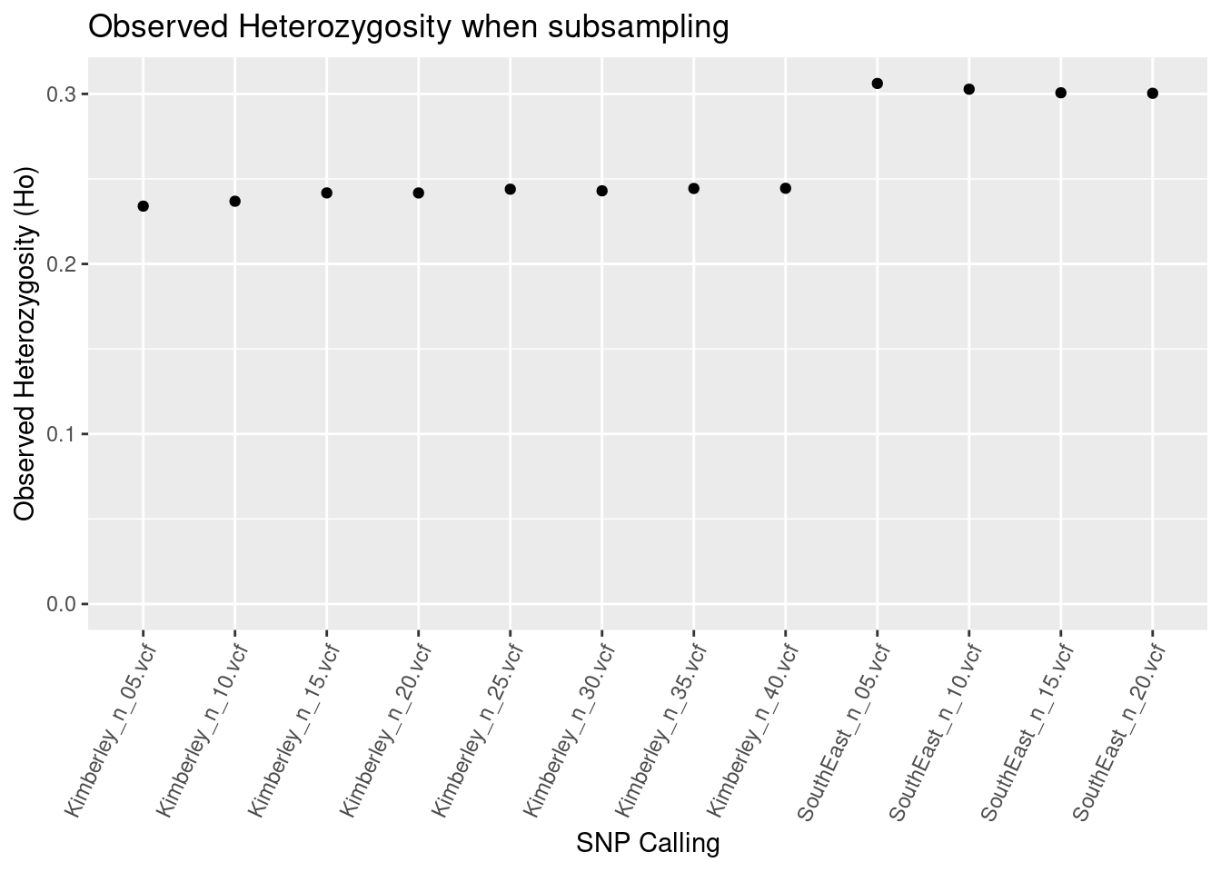
central_Ho_subsampling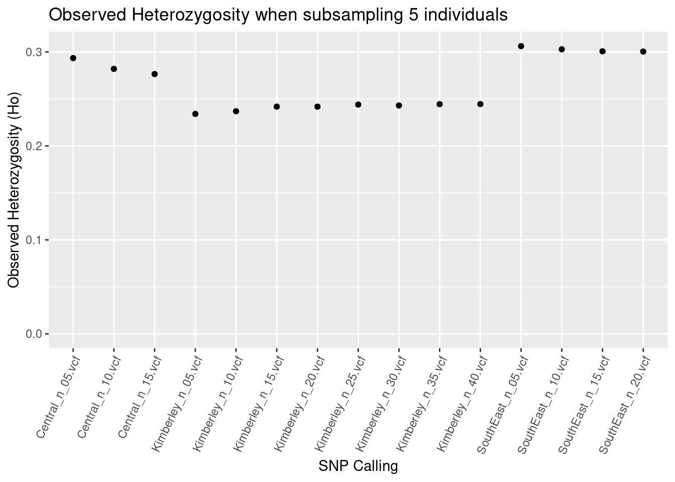
Subsampling
So we’re not seeing too much impact of subsampling if SNPs are called separately on populations.
BUT, BUT, BUT, BUT, BUT, BUT, BUT…
The Kimberley population has the highest actual heterozygosity (see the paper). The difference here is that this population lost a lot of variable sites because more than 5% (or >35k) of the variable sites have more than two alleles. So a comparison between Central, Southeast and Kimberley Litoria rubella would find the highest heterozygosity in the wrong population.
This is very problematic and is an ongoing bioinformatic issue.
Therefore, calling SNPs separately on populations and keeping sample sizes the same does not resolve the issues with heterozygosity based on SNPs.
Calling populations together
Does this resolve the issue?
Lets look at a file where SNPs were called on all three populations at once, and the samples were equal numbers.
#first we assign populations to the individuals in the genlight
individual_names <- as.vector(indNames(combined_kim_15_cen_15_se_15.vcf))

# Split each name at the underscore and keep the first part
modified_names <- sapply(individual_names, function(name) {
  parts <- strsplit(name, "_")[[1]]
  parts[1]
})

# Convert the output to a factor
modified_names <- factor(modified_names)

#then we assign the populations
combined_kim_15_cen_15_se_15.vcf@pop <- modified_names

#then we apply a call rate filter
combined_kim_15_cen_15_se_15.vcf_0.7 <- gl.filter.callrate(combined_kim_15_cen_15_se_15.vcf,
                                                           threshold = 0.95, mono.rm = T)
Starting gl.filter.callrate
Processing genlight object with SNP data
Warning: Data may include monomorphic loci in call rate
calculations for filtering
Recalculating Call Rate
Removing loci based on Call Rate, threshold = 0.95 
Completed: gl.filter.callrate #then we look at the heterozygosity estimates by population
diversity_equal_sample_15_ind <- gl.report.heterozygosity(combined_kim_15_cen_15_se_15.vcf_0.7)Starting gl.report.heterozygosity
Processing genlight object with SNP data
Calculating Observed Heterozygosities, averaged across
loci, for each population
Calculating Expected Heterozygosities
Starting gl.colors
Selected color type dis
Completed: gl.colors 
                pop    n.Ind n.Loc n.Loc.adj polyLoc monoLoc all_NALoc       Ho
Central     Central 14.74289   914         1     205     709         0 0.037671
Kimberley Kimberley 14.07878   914         1     656     258         0 0.117284
SouthEast SouthEast 14.62144   914         1     372     542         0 0.079583
              HoSD     HoSE HoLCI HoHCI   Ho.adj Ho.adjSD Ho.adjSE Ho.adjLCI
Central   0.112102 0.003708    NA    NA 0.037671 0.112102 0.003708        NA
Kimberley 0.134002 0.004432    NA    NA 0.117284 0.134002 0.004432        NA
SouthEast 0.134695 0.004455    NA    NA 0.079583 0.134695 0.004455        NA
          Ho.adjHCI       He     HeSD     HeSE HeLCI HeHCI      uHe    uHeSD
Central          NA 0.071363 0.153583 0.005080    NA    NA 0.073868 0.158975
Kimberley        NA 0.143542 0.152636 0.005049    NA    NA 0.148827 0.158257
SouthEast        NA 0.089745 0.145624 0.004817    NA    NA 0.092922 0.150781
             uHeSE uHeLCI uHeHCI   He.adj He.adjSD He.adjSE He.adjLCI He.adjHCI
Central   0.005258     NA     NA 0.071363 0.153583 0.005080        NA        NA
Kimberley 0.005235     NA     NA 0.143542 0.152636 0.005049        NA        NA
SouthEast 0.004987     NA     NA 0.089745 0.145624 0.004817        NA        NA
               FIS    FISSD    FISSE FISLCI FISHCI
Central   0.400900 0.452247 0.014959     NA     NA
Kimberley 0.128504 0.310302 0.010264     NA     NA
SouthEast 0.091166 0.254158 0.008407     NA     NA
Completed: gl.report.heterozygosity
We now see that our heterozygosity is found to be highest in the Kimberley and lowest in Central Australia, which is true.
Calling SNPs together but with different sample sizes
Lots of times we have different numbers of samples… so what does this do to our estimates? Lets look at what happens when we have different sample numbers across all populations
individual_names <- as.vector(indNames(combined_kim_15_cen_5_se_10.vcf))

# Split each name at the underscore and keep the first part
modified_names <- sapply(individual_names, function(name) {
  parts <- strsplit(name, "_")[[1]]
  parts[1]
})

# Convert the output to a factor
modified_names <- factor(modified_names)

#then we assign the populations
combined_kim_15_cen_5_se_10.vcf@pop <- modified_names

#then we apply a call rate filter
combined_kim_15_cen_5_se_10.vcf_0.95 <- gl.filter.callrate(combined_kim_15_cen_5_se_10.vcf, threshold = 0.95, mono.rm = T)
Starting gl.filter.callrate
Processing genlight object with SNP data
Warning: Data may include monomorphic loci in call rate
calculations for filtering
Recalculating Call Rate
Removing loci based on Call Rate, threshold = 0.95 
Completed: gl.filter.callrate #then we look at the heterozygosity estimates by population
diversity_unequal_sample <- gl.report.heterozygosity(combined_kim_15_cen_5_se_10.vcf_0.95)Starting gl.report.heterozygosity
Processing genlight object with SNP data
Calculating Observed Heterozygosities, averaged across
loci, for each population
Calculating Expected Heterozygosities
Starting gl.colors
Selected color type dis
Completed: gl.colors 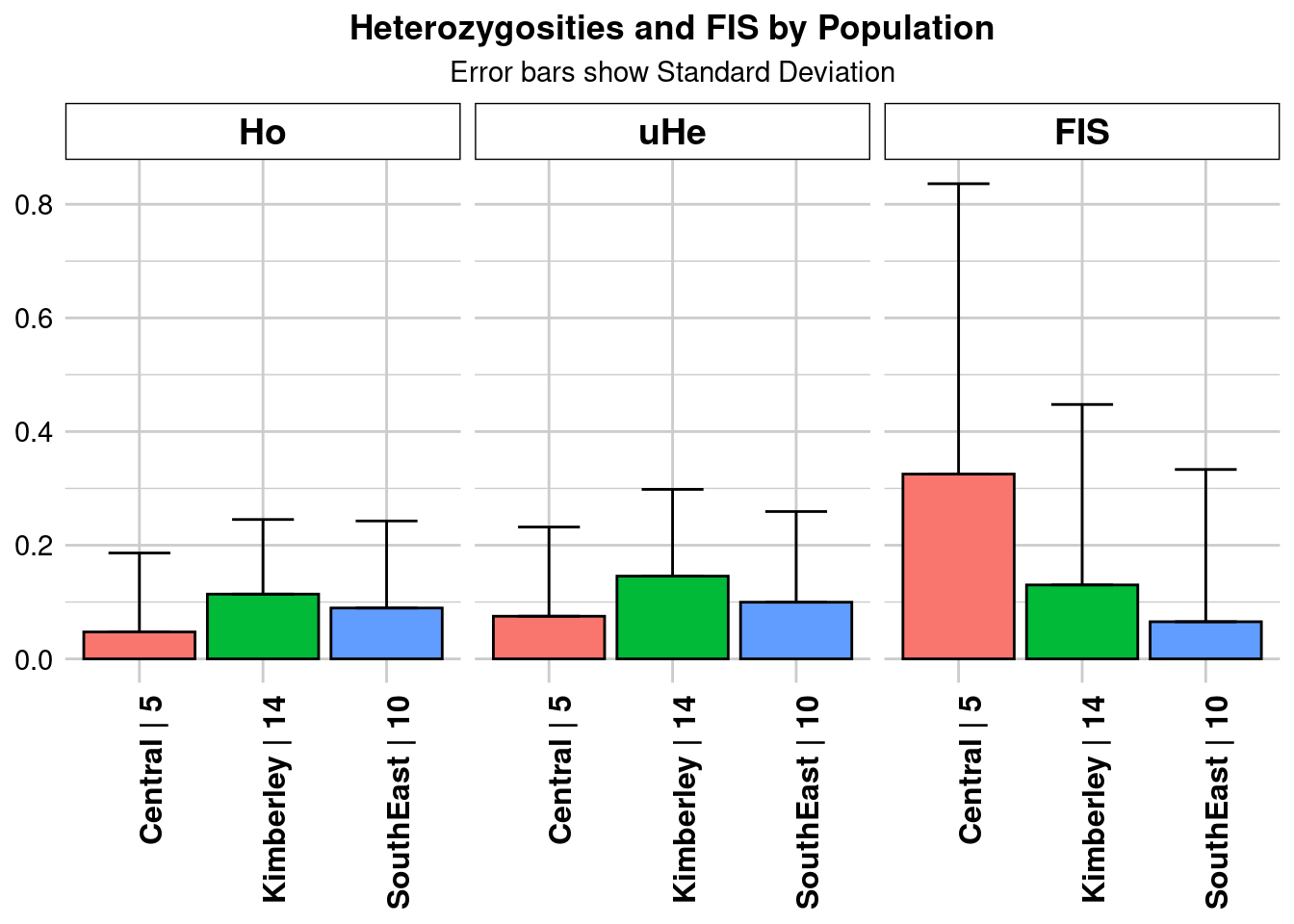
                pop     n.Ind n.Loc n.Loc.adj polyLoc monoLoc all_NALoc
Central     Central  4.980290   964         1     206     758         0
Kimberley Kimberley 14.429461   964         1     709     255         0
SouthEast SouthEast  9.854772   964         1     373     591         0
                Ho     HoSD     HoSE HoLCI HoHCI   Ho.adj Ho.adjSD Ho.adjSE
Central   0.047355 0.138961 0.004476    NA    NA 0.047355 0.138961 0.004476
Kimberley 0.113975 0.131324 0.004230    NA    NA 0.113975 0.131324 0.004230
SouthEast 0.089523 0.153169 0.004933    NA    NA 0.089523 0.153169 0.004933
          Ho.adjLCI Ho.adjHCI       He     HeSD     HeSE HeLCI HeHCI      uHe
Central          NA        NA 0.067501 0.141209 0.004548    NA    NA 0.075034
Kimberley        NA        NA 0.140553 0.147435 0.004749    NA    NA 0.145598
SouthEast        NA        NA 0.094679 0.151447 0.004878    NA    NA 0.099740
             uHeSD    uHeSE uHeLCI uHeHCI   He.adj He.adjSD He.adjSE He.adjLCI
Central   0.156968 0.005056     NA     NA 0.067501 0.141209 0.004548        NA
Kimberley 0.152727 0.004919     NA     NA 0.140553 0.147435 0.004749        NA
SouthEast 0.159541 0.005138     NA     NA 0.094679 0.151447 0.004878        NA
          He.adjHCI      FIS    FISSD    FISSE FISLCI FISHCI
Central          NA 0.325189 0.510923 0.016456     NA     NA
Kimberley        NA 0.130096 0.317600 0.010229     NA     NA
SouthEast        NA 0.065369 0.267902 0.008629     NA     NA
Completed: gl.report.heterozygosity
#how much more heterozygosity does kimberley have than central in different analyses?
#where our samples are equal?
diversity_equal_sample_15_ind$Ho[1]/diversity_equal_sample_15_ind$Ho[3][1] 0.4733549#where our samples are equal?
diversity_unequal_sample$Ho[1]/diversity_unequal_sample$Ho[3][1] 0.5289702
Take away
What you need to take away is that as the sample size of our most diverse population grows, the less diverse populations become more similar. In this case, if you use really unequal sample sizes, your results get so biased that your less diverse population can be calculated as more diverse than your most diverse population.
Think of the conservation implications!
In a full analysis of all the data, with unequal sample numbers and SNPs called on all populations, we got a result that the Kimberley population was the least diverse. This would then result in a direction that the most genetically important population is actually one of the least.
SNP-based heterozygosity
SNP-based heterozygosity is extremely biased and cannot be used to compare different populations, and there are no clear workarounds that will give you reliable answers.
You need to report autosomal heterozygosity at a minimum, which means doing your own bioinformatics from raw data at this time.
Further Study
Galaxy Australia:
Bioinformatics resources available to through the AAF login (your university)
Lots of compute power
Has the Stacks2 pipeline available
Links:
https://australianbiocommons.github.io/how-to-guides/stacks_workflows/stacks