10 Sex Linked Markers

Session presenters

Required packages

library(dartR.base)
library(dartR.sexlinked)

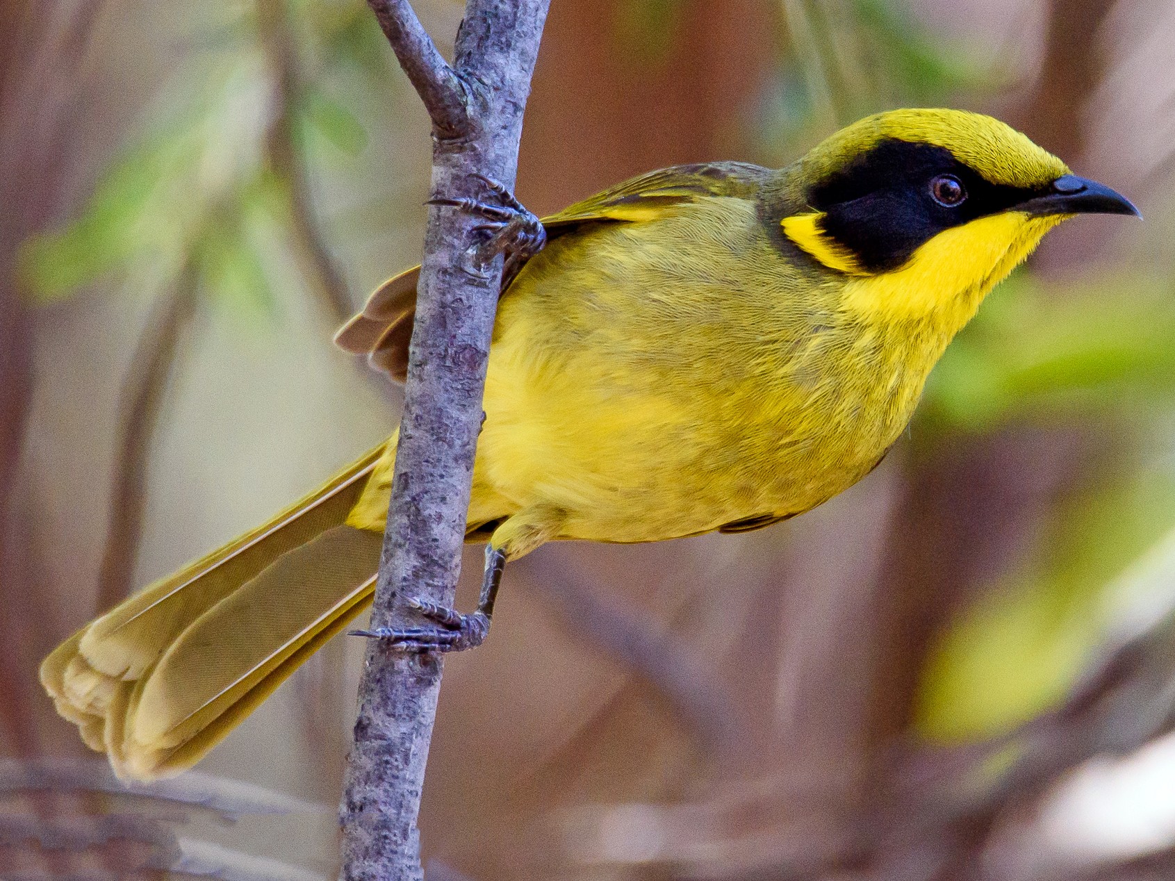
Dataset 1 - ZW//ZZ - The Yellow Tufted Honeyeater

Load data

#data("YTH")
load('./data/YTH.rda')
YTH                   # Explore the dataset

 ********************
 *** DARTR OBJECT ***
 ********************

 ** 609 genotypes,  994 SNPs , size: 49.9 Mb

    missing data: 139174 (=22.99 %) scored as NA

 ** Genetic data
   @gen: list of 609 SNPbin
   @ploidy: ploidy of each individual  (range: 2-2)

 ** Additional data
   @ind.names:  609 individual labels
   @loc.names:  994 locus labels
   @loc.all:  994 allele labels
   @position: integer storing positions of the SNPs [within 69 base sequence]
   @pop: population of each individual (group size range: 12-516)
   @other: a list containing: loc.metrics, ind.metrics, loc.metrics.flags, verbose, history 
    @other$ind.metrics: id, pop, sex, sex_original, service, plate_location 
    @other$loc.metrics: AlleleID, CloneID, AlleleSequence, TrimmedSequence, Chrom_Lichenostomus_HeHo_v1, ChromPos_Lichenostomus_HeHo_v1, AlnCnt_Lichenostomus_HeHo_v1, AlnEvalue_Lichenostomus_HeHo_v1, SNP, SnpPosition, CallRate, OneRatioRef, OneRatioSnp, FreqHomRef, FreqHomSnp, FreqHets, PICRef, PICSnp, AvgPIC, AvgCountRef, AvgCountSnp, RepAvg, clone, uid, rdepth, maf 
   @other$latlon[g]: no coordinates attached

YTH@n.loc             # Number of SNPs

[1] 994

length(YTH@ind.names) # Number of individuals

[1] 609

Run `gl.filter.sexlinked`

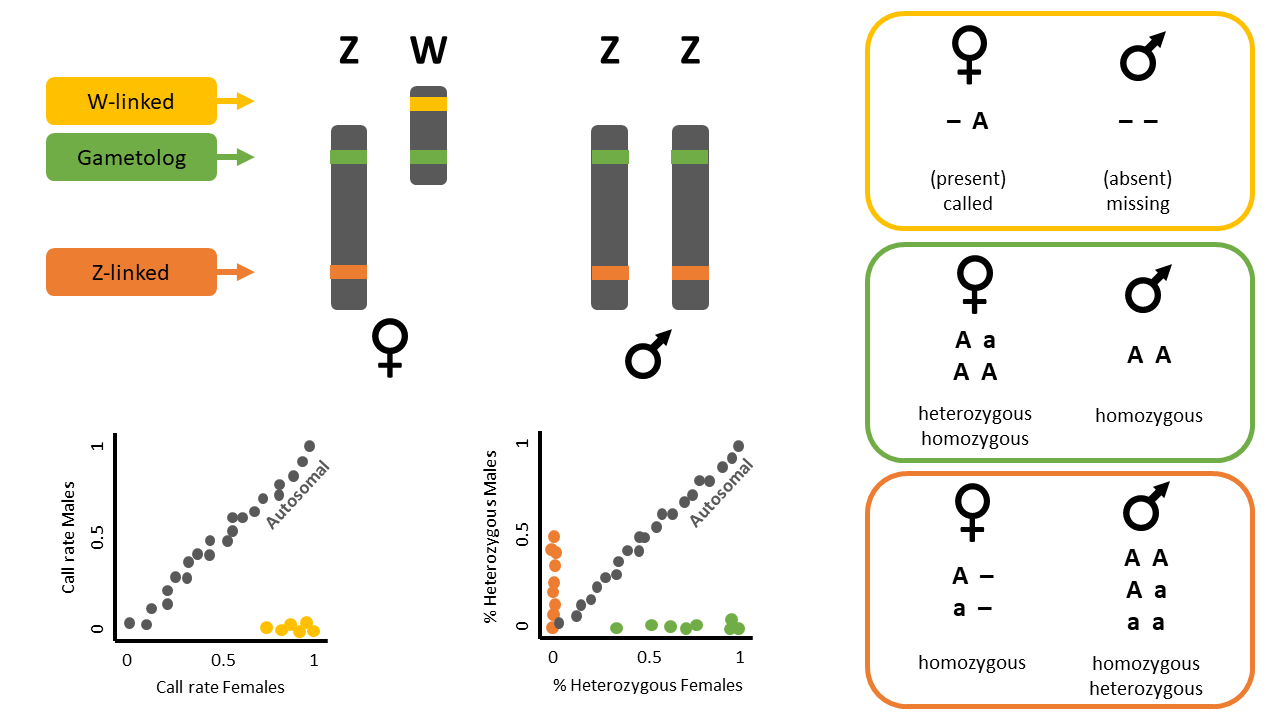
This function identifies sex-linked and autosomal loci present in a SNP dataset (i.e., genlight object) using individuals with known sex. It identifies five types of loci: w-linked or y-linked, sex-biased, z-linked or x-linked, gametologous and autosomal.

The genlight object must contain in gl@other$ind.metrics a column named “id”, and a column named “sex” in which individuals with known-sex are assigned ‘M’ for male, or ‘F’ for female. The function ignores individuals that are assigned anything else or nothing at all (unknown-sex).

Caution

NOTE

Set ncores to more than 1 (default) if you have more than 50,000 SNPs, since it could actually slow down the analysis with smaller datasets.

knitr::kable(head(YTH@other$ind.metrics)) # Check that ind.metrics has the necessary columns

	id	pop	sex	sex_original	service	plate_location
ANWC46839	ANWC46839	Melanops	F	F	DLich17-2918	1-A1
W49	W49	Cassidix	F	F	DLich17-2918	1-A10
W90	W90	Cassidix	F	F	DLich17-2918	1-A12
C25	C25	Cassidix	M	M	DLich17-2918	1-A2
C8	C8	Cassidix	M	M	DLich17-2918	1-A3
W70	W70	Cassidix	F	F	DLich17-2918	1-A4

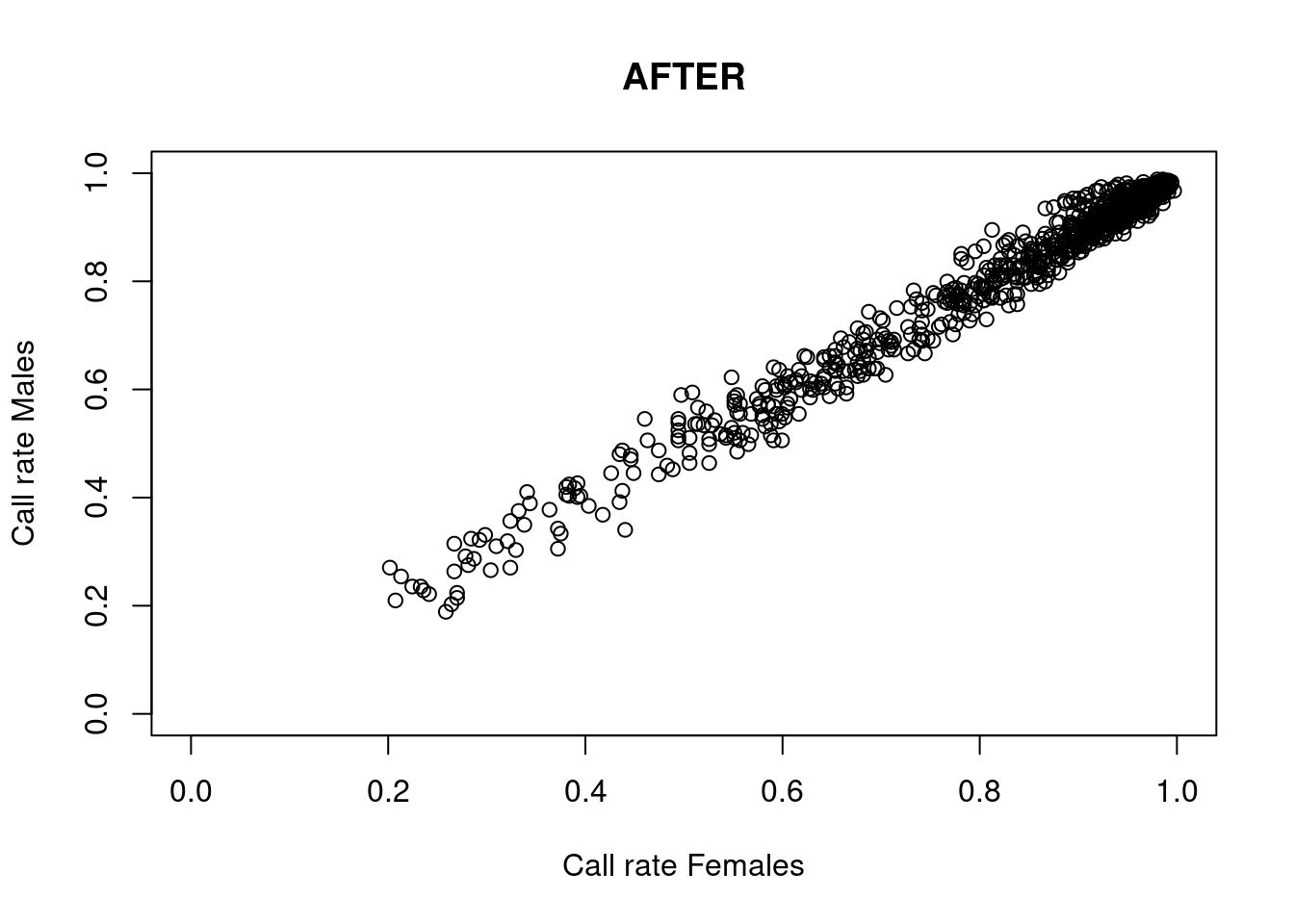
res <- dartR.sexlinked::gl.filter.sexlinked(gl = YTH, system = "zw")

Detected 276 females and 333 males.

Starting phase 1. May take a while...

Building call rate plots.

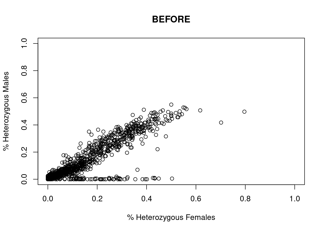
Done. Starting phase 2.

Building heterozygosity plots.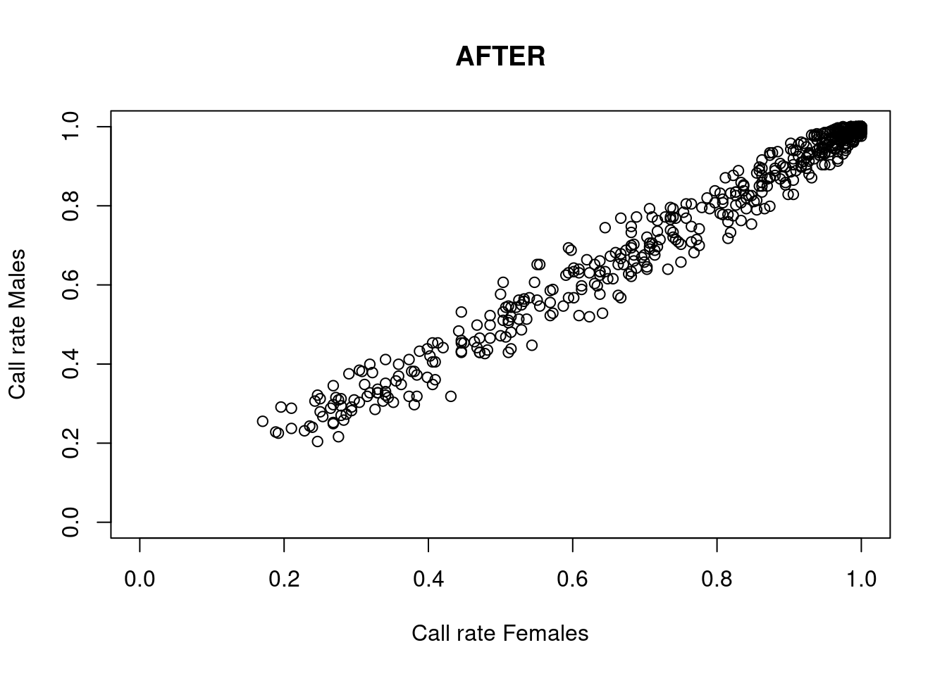

Done building heterozygosity plots.

**FINISHED** Total of analyzed loci: 994.
Found 506 sex-linked loci:
   52 W-linked loci
   273 sex-biased loci
   165 Z-linked loci
   16 ZW gametologs.
And 488 autosomal loci.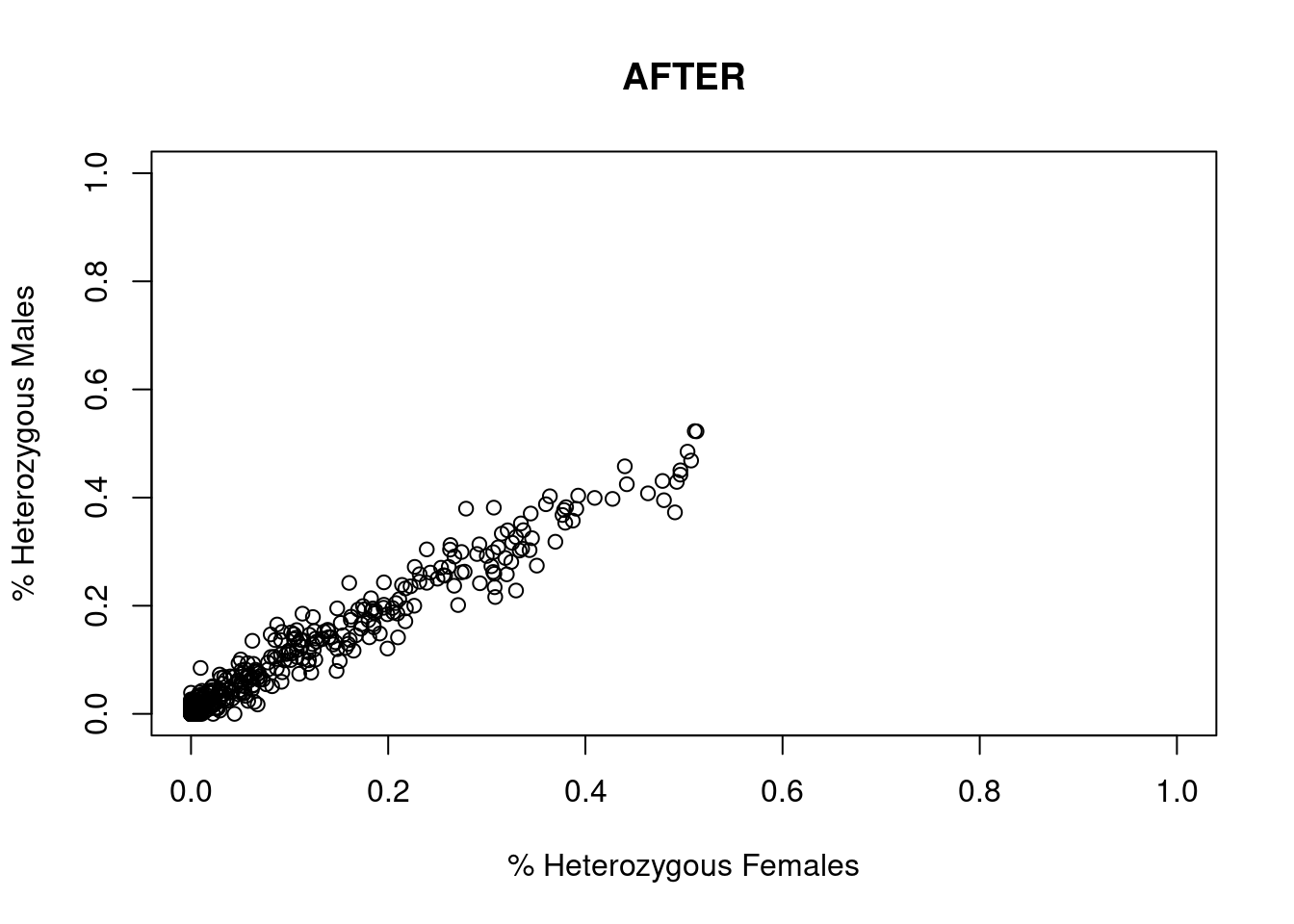

Exercise

How many males and females does the dataset contain?

How many sex-linked loci were found?

Now check the output:

res$w.linked       # Notice that it says "w-linked"

 ********************
 *** DARTR OBJECT ***
 ********************

 ** 609 genotypes,  52 SNPs , size: 48.9 Mb

    missing data: 17304 (=54.64 %) scored as NA

 ** Genetic data
   @gen: list of 609 SNPbin
   @ploidy: ploidy of each individual  (range: 2-2)

 ** Additional data
   @ind.names:  609 individual labels
   @loc.names:  52 locus labels
   @loc.all:  52 allele labels
   @position: integer storing positions of the SNPs [within 69 base sequence]
   @pop: population of each individual (group size range: 12-516)
   @other: a list containing: loc.metrics, ind.metrics, loc.metrics.flags, verbose, history 
    @other$ind.metrics: id, pop, sex, sex_original, service, plate_location 
    @other$loc.metrics: AlleleID, CloneID, AlleleSequence, TrimmedSequence, Chrom_Lichenostomus_HeHo_v1, ChromPos_Lichenostomus_HeHo_v1, AlnCnt_Lichenostomus_HeHo_v1, AlnEvalue_Lichenostomus_HeHo_v1, SNP, SnpPosition, CallRate, OneRatioRef, OneRatioSnp, FreqHomRef, FreqHomSnp, FreqHets, PICRef, PICSnp, AvgPIC, AvgCountRef, AvgCountSnp, RepAvg, clone, uid, rdepth, maf 
   @other$latlon[g]: no coordinates attached

res$z.linked       # Notice that it says "z-linked"

 ********************
 *** DARTR OBJECT ***
 ********************

 ** 609 genotypes,  165 SNPs , size: 48.9 Mb

    missing data: 2990 (=2.98 %) scored as NA

 ** Genetic data
   @gen: list of 609 SNPbin
   @ploidy: ploidy of each individual  (range: 2-2)

 ** Additional data
   @ind.names:  609 individual labels
   @loc.names:  165 locus labels
   @loc.all:  165 allele labels
   @position: integer storing positions of the SNPs [within 69 base sequence]
   @pop: population of each individual (group size range: 12-516)
   @other: a list containing: loc.metrics, ind.metrics, loc.metrics.flags, verbose, history 
    @other$ind.metrics: id, pop, sex, sex_original, service, plate_location 
    @other$loc.metrics: AlleleID, CloneID, AlleleSequence, TrimmedSequence, Chrom_Lichenostomus_HeHo_v1, ChromPos_Lichenostomus_HeHo_v1, AlnCnt_Lichenostomus_HeHo_v1, AlnEvalue_Lichenostomus_HeHo_v1, SNP, SnpPosition, CallRate, OneRatioRef, OneRatioSnp, FreqHomRef, FreqHomSnp, FreqHets, PICRef, PICSnp, AvgPIC, AvgCountRef, AvgCountSnp, RepAvg, clone, uid, rdepth, maf 
   @other$latlon[g]: no coordinates attached

res$gametolog

 ********************
 *** DARTR OBJECT ***
 ********************

 ** 609 genotypes,  16 SNPs , size: 48.8 Mb

    missing data: 580 (=5.95 %) scored as NA

 ** Genetic data
   @gen: list of 609 SNPbin
   @ploidy: ploidy of each individual  (range: 2-2)

 ** Additional data
   @ind.names:  609 individual labels
   @loc.names:  16 locus labels
   @loc.all:  16 allele labels
   @position: integer storing positions of the SNPs [within 69 base sequence]
   @pop: population of each individual (group size range: 12-516)
   @other: a list containing: loc.metrics, ind.metrics, loc.metrics.flags, verbose, history 
    @other$ind.metrics: id, pop, sex, sex_original, service, plate_location 
    @other$loc.metrics: AlleleID, CloneID, AlleleSequence, TrimmedSequence, Chrom_Lichenostomus_HeHo_v1, ChromPos_Lichenostomus_HeHo_v1, AlnCnt_Lichenostomus_HeHo_v1, AlnEvalue_Lichenostomus_HeHo_v1, SNP, SnpPosition, CallRate, OneRatioRef, OneRatioSnp, FreqHomRef, FreqHomSnp, FreqHets, PICRef, PICSnp, AvgPIC, AvgCountRef, AvgCountSnp, RepAvg, clone, uid, rdepth, maf 
   @other$latlon[g]: no coordinates attached

res$sex.biased

 ********************
 *** DARTR OBJECT ***
 ********************

 ** 609 genotypes,  273 SNPs , size: 49.2 Mb

    missing data: 46048 (=27.7 %) scored as NA

 ** Genetic data
   @gen: list of 609 SNPbin
   @ploidy: ploidy of each individual  (range: 2-2)

 ** Additional data
   @ind.names:  609 individual labels
   @loc.names:  273 locus labels
   @loc.all:  273 allele labels
   @position: integer storing positions of the SNPs [within 69 base sequence]
   @pop: population of each individual (group size range: 12-516)
   @other: a list containing: loc.metrics, ind.metrics, loc.metrics.flags, verbose, history 
    @other$ind.metrics: id, pop, sex, sex_original, service, plate_location 
    @other$loc.metrics: AlleleID, CloneID, AlleleSequence, TrimmedSequence, Chrom_Lichenostomus_HeHo_v1, ChromPos_Lichenostomus_HeHo_v1, AlnCnt_Lichenostomus_HeHo_v1, AlnEvalue_Lichenostomus_HeHo_v1, SNP, SnpPosition, CallRate, OneRatioRef, OneRatioSnp, FreqHomRef, FreqHomSnp, FreqHets, PICRef, PICSnp, AvgPIC, AvgCountRef, AvgCountSnp, RepAvg, clone, uid, rdepth, maf 
   @other$latlon[g]: no coordinates attached

res$autosomal

 ********************
 *** DARTR OBJECT ***
 ********************

 ** 609 genotypes,  488 SNPs , size: 49.4 Mb

    missing data: 72252 (=24.31 %) scored as NA

 ** Genetic data
   @gen: list of 609 SNPbin
   @ploidy: ploidy of each individual  (range: 2-2)

 ** Additional data
   @ind.names:  609 individual labels
   @loc.names:  488 locus labels
   @loc.all:  488 allele labels
   @position: integer storing positions of the SNPs [within 69 base sequence]
   @pop: population of each individual (group size range: 12-516)
   @other: a list containing: loc.metrics, ind.metrics, loc.metrics.flags, verbose, history 
    @other$ind.metrics: id, pop, sex, sex_original, service, plate_location 
    @other$loc.metrics: AlleleID, CloneID, AlleleSequence, TrimmedSequence, Chrom_Lichenostomus_HeHo_v1, ChromPos_Lichenostomus_HeHo_v1, AlnCnt_Lichenostomus_HeHo_v1, AlnEvalue_Lichenostomus_HeHo_v1, SNP, SnpPosition, CallRate, OneRatioRef, OneRatioSnp, FreqHomRef, FreqHomSnp, FreqHets, PICRef, PICSnp, AvgPIC, AvgCountRef, AvgCountSnp, RepAvg, clone, uid, rdepth, maf 
   @other$latlon[g]: no coordinates attached

knitr::kable(head(res$results.table))  # The output table

	index	count.F.miss	count.M.miss	count.F.scored	count.M.scored	ratio	p.value	p.adjusted	scoringRate.F	scoringRate.M	w.linked	sex.biased	count.F.het	count.M.het	count.F.hom	count.M.hom	stat	stat.p.value	stat.p.adjusted	heterozygosity.F	heterozygosity.M	z.linked	zw.gametolog
27382025-26-T/C	1	61	25	215	308	3.4882302	0.0000003	0.0000016	0.7789855	0.9249249	FALSE	TRUE	0	73	215	235	NA	NA	NA	0.0000000	0.2370130	FALSE	FALSE
27338005-34-A/G	2	12	13	264	320	1.1186728	0.8390268	1.0000000	0.9565217	0.9609610	FALSE	FALSE	0	144	264	176	0.0046581	0.0000000	0.0000000	0.0000000	0.4500000	TRUE	FALSE
27331627-16-T/G	3	108	159	168	174	0.7039235	0.0334301	0.0860868	0.6086957	0.5225225	FALSE	FALSE	0	2	168	172	0.5128690	1.0000000	1.0000000	0.0000000	0.0114943	FALSE	FALSE
53948461-35-G/A	4	46	64	230	269	0.8408645	0.4593502	0.7791707	0.8333333	0.8078078	FALSE	FALSE	29	27	201	242	1.2924846	0.3950852	0.9051780	0.1260870	0.1003717	FALSE	FALSE
27360874-8-A/G	5	41	63	235	270	0.7480768	0.1956613	0.4120495	0.8514493	0.8108108	FALSE	FALSE	25	38	210	232	0.7272744	0.2807852	0.7009152	0.1063830	0.1407407	FALSE	FALSE
27377678-32-C/A	6	30	33	246	300	1.1084581	0.7894511	1.0000000	0.8913043	0.9009009	FALSE	FALSE	3	6	243	294	0.6054740	0.5234966	1.0000000	0.0121951	0.0200000	FALSE	FALSE

The output consists of a genlight object for each type of loci, plus a results table.

Run `gl.infer.sex`

This function uses the complete output of function gl.filter.sexlinked (list of 6 objects) to infer the sex of all individuals in the dataset. Specifically, the function uses 3 types of sex-linked loci (W-/Y-linked, Z-/X-linked, and gametologs), assigns a preliminary genetic sex for each type of sex-linked loci available, and outputs an agreed sex.

sexID <- dartR.sexlinked::gl.infer.sex(gl_sex_filtered = res, system = "zw", seed = 124)

***FINISHED***

knitr::kable(head(sexID))

	id	w.linked.sex	#missing	#called	z.linked.sex	#Hom.z	#Het.z	gametolog.sex	#Hom.g	#Het.g	agreed.sex
ANWC46839	ANWC46839	F	51	1	F	1	141	F	5	0	F
W49	W49	F	52	0	F	2	156	F	5	0	F
W90	W90	F	48	4	F	0	162	F	5	0	F
C25	C25	M	0	52	M	52	113	M	0	5	M
C8	C8	M	0	52	M	48	116	M	0	5	M
W70	W70	F	49	3	F	0	152	F	5	0	F

Warning

IMPORTANT We created this function with the explicit intent that a human checks the evidence for the agreed sex that do NOT agree for all types of sex-linked loci (denoted as ‘*M’ or ‘*F’). This human can then use their criterion to validate these assignments.

Exercise

Can you find individuals for which the agreed sex is uncertain (i.e., has an asterisk “*”)?

Dataset 2 - XX/XY - The Leadbeater’s possum

Load data

#data("LBP")
load('./data/LBP.rda')
LBP                   # Explore the dataset

 ********************
 *** DARTR OBJECT ***
 ********************

 ** 376 genotypes,  1,000 SNPs , size: 5.2 Mb

    missing data: 20670 (=5.5 %) scored as NA

 ** Genetic data
   @gen: list of 376 SNPbin
   @ploidy: ploidy of each individual  (range: 2-2)

 ** Additional data
   @ind.names:  376 individual labels
   @loc.names:  1000 locus labels
   @loc.all:  1000 allele labels
   @position: integer storing positions of the SNPs [within 69 base sequence]
   @pop: population of each individual (group size range: 95-281)
   @other: a list containing: loc.metrics, ind.metrics, loc.metrics.flags, verbose, history 
    @other$ind.metrics: id, sex, pop, Year.collected, service, plate_location 
    @other$loc.metrics: AlleleID, CloneID, AlleleSequence, TrimmedSequence, Chrom_Possum_v2, ChromPos_Possum_v2, AlnCnt_Possum_v2, AlnEvalue_Possum_v2, SNP, SnpPosition, CallRate, OneRatioRef, OneRatioSnp, FreqHomRef, FreqHomSnp, FreqHets, PICRef, PICSnp, AvgPIC, AvgCountRef, AvgCountSnp, RepAvg, clone, uid, rdepth, monomorphs, maf, OneRatio, PIC 
   @other$latlon[g]: no coordinates attached

LBP@n.loc             # Number of SNPs

[1] 1000

length(LBP@ind.names) # Number of individuals

[1] 376

Run `gl.filter.sexlinked`

This function identifies sex-linked and autosomal loci present in a SNP dataset (genlight object) using individuals with known sex. It identifies five types of loci: w-linked or y-linked, sex-biased, z-linked or x-linked, gametologous and autosomal.

knitr::kable(head(LBP@other$ind.metrics)) # Check that ind.metrics has the necessary columns

	id	sex	pop	Year.collected	service	plate_location
Y2	Y2	F	Yellingbo	1997	DLpos17-2786	1-A1
Y16	Y16	M	Yellingbo	2001	DLpos17-2786	1-A10
Y17	Y17	F	Yellingbo	1997	DLpos17-2786	1-A11
Y18	Y18	F	Yellingbo	1999	DLpos17-2786	1-A12
Y3	Y3	F	Yellingbo	1997	DLpos17-2786	1-A2
Y4	Y4	M	Yellingbo	1997	DLpos17-2786	1-A3

res <- dartR.sexlinked::gl.filter.sexlinked(gl = LBP, system = "xy")

Detected 162 females and 211 males.

Starting phase 1. May take a while...

Building call rate plots.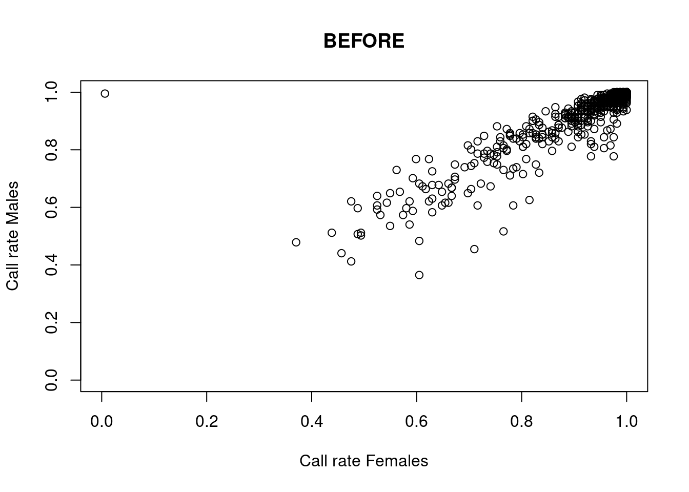

Done. Starting phase 2.

Building heterozygosity plots.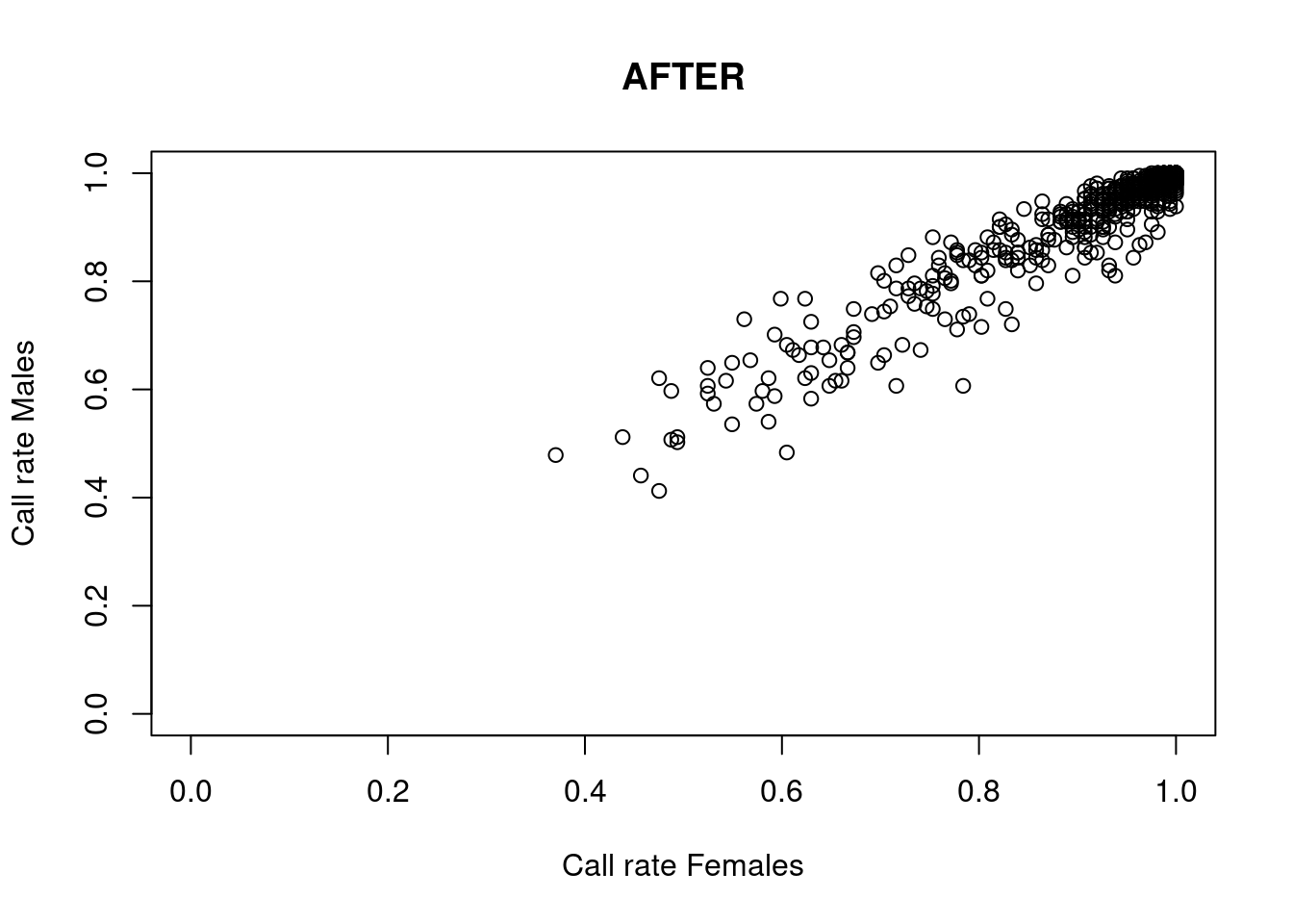

Done building heterozygosity plots.

**FINISHED** Total of analyzed loci: 1000.
Found 77 sex-linked loci:
   1 Y-linked loci
   9 sex-biased loci
   66 X-linked loci
   1 XY gametologs.
And 923 autosomal loci.

Exercise

How many males and females does the dataset contain?

How many sex-linked loci were found?

Now check the output:

res$y.linked      # Notice that it says "y-linked"

 ********************
 *** DARTR OBJECT ***
 ********************

 ** 376 genotypes,  1 SNPs , size: 4.7 Mb

    missing data: 164 (=43.62 %) scored as NA

 ** Genetic data
   @gen: list of 376 SNPbin
   @ploidy: ploidy of each individual  (range: 2-2)

 ** Additional data
   @ind.names:  376 individual labels
   @loc.names:  1 locus labels
   @loc.all:  1 allele labels
   @position: integer storing positions of the SNPs [within 69 base sequence]
   @pop: population of each individual (group size range: 95-281)
   @other: a list containing: loc.metrics, ind.metrics, loc.metrics.flags, verbose, history 
    @other$ind.metrics: id, sex, pop, Year.collected, service, plate_location 
    @other$loc.metrics: AlleleID, CloneID, AlleleSequence, TrimmedSequence, Chrom_Possum_v2, ChromPos_Possum_v2, AlnCnt_Possum_v2, AlnEvalue_Possum_v2, SNP, SnpPosition, CallRate, OneRatioRef, OneRatioSnp, FreqHomRef, FreqHomSnp, FreqHets, PICRef, PICSnp, AvgPIC, AvgCountRef, AvgCountSnp, RepAvg, clone, uid, rdepth, monomorphs, maf, OneRatio, PIC 
   @other$latlon[g]: no coordinates attached

res$x.linked      # Notice that it says "x-linked"

 ********************
 *** DARTR OBJECT ***
 ********************

 ** 376 genotypes,  66 SNPs , size: 4.7 Mb

    missing data: 827 (=3.33 %) scored as NA

 ** Genetic data
   @gen: list of 376 SNPbin
   @ploidy: ploidy of each individual  (range: 2-2)

 ** Additional data
   @ind.names:  376 individual labels
   @loc.names:  66 locus labels
   @loc.all:  66 allele labels
   @position: integer storing positions of the SNPs [within 69 base sequence]
   @pop: population of each individual (group size range: 95-281)
   @other: a list containing: loc.metrics, ind.metrics, loc.metrics.flags, verbose, history 
    @other$ind.metrics: id, sex, pop, Year.collected, service, plate_location 
    @other$loc.metrics: AlleleID, CloneID, AlleleSequence, TrimmedSequence, Chrom_Possum_v2, ChromPos_Possum_v2, AlnCnt_Possum_v2, AlnEvalue_Possum_v2, SNP, SnpPosition, CallRate, OneRatioRef, OneRatioSnp, FreqHomRef, FreqHomSnp, FreqHets, PICRef, PICSnp, AvgPIC, AvgCountRef, AvgCountSnp, RepAvg, clone, uid, rdepth, monomorphs, maf, OneRatio, PIC 
   @other$latlon[g]: no coordinates attached

res$gametolog

 ********************
 *** DARTR OBJECT ***
 ********************

 ** 376 genotypes,  1 SNPs , size: 4.7 Mb

    missing data: 0 (=0 %) scored as NA

 ** Genetic data
   @gen: list of 376 SNPbin
   @ploidy: ploidy of each individual  (range: 2-2)

 ** Additional data
   @ind.names:  376 individual labels
   @loc.names:  1 locus labels
   @loc.all:  1 allele labels
   @position: integer storing positions of the SNPs [within 69 base sequence]
   @pop: population of each individual (group size range: 95-281)
   @other: a list containing: loc.metrics, ind.metrics, loc.metrics.flags, verbose, history 
    @other$ind.metrics: id, sex, pop, Year.collected, service, plate_location 
    @other$loc.metrics: AlleleID, CloneID, AlleleSequence, TrimmedSequence, Chrom_Possum_v2, ChromPos_Possum_v2, AlnCnt_Possum_v2, AlnEvalue_Possum_v2, SNP, SnpPosition, CallRate, OneRatioRef, OneRatioSnp, FreqHomRef, FreqHomSnp, FreqHets, PICRef, PICSnp, AvgPIC, AvgCountRef, AvgCountSnp, RepAvg, clone, uid, rdepth, monomorphs, maf, OneRatio, PIC 
   @other$latlon[g]: no coordinates attached

res$sex.biased

 ********************
 *** DARTR OBJECT ***
 ********************

 ** 376 genotypes,  9 SNPs , size: 4.7 Mb

    missing data: 853 (=25.21 %) scored as NA

 ** Genetic data
   @gen: list of 376 SNPbin
   @ploidy: ploidy of each individual  (range: 2-2)

 ** Additional data
   @ind.names:  376 individual labels
   @loc.names:  9 locus labels
   @loc.all:  9 allele labels
   @position: integer storing positions of the SNPs [within 69 base sequence]
   @pop: population of each individual (group size range: 95-281)
   @other: a list containing: loc.metrics, ind.metrics, loc.metrics.flags, verbose, history 
    @other$ind.metrics: id, sex, pop, Year.collected, service, plate_location 
    @other$loc.metrics: AlleleID, CloneID, AlleleSequence, TrimmedSequence, Chrom_Possum_v2, ChromPos_Possum_v2, AlnCnt_Possum_v2, AlnEvalue_Possum_v2, SNP, SnpPosition, CallRate, OneRatioRef, OneRatioSnp, FreqHomRef, FreqHomSnp, FreqHets, PICRef, PICSnp, AvgPIC, AvgCountRef, AvgCountSnp, RepAvg, clone, uid, rdepth, monomorphs, maf, OneRatio, PIC 
   @other$latlon[g]: no coordinates attached

res$autosomal

 ********************
 *** DARTR OBJECT ***
 ********************

 ** 376 genotypes,  923 SNPs , size: 5.2 Mb

    missing data: 18826 (=5.42 %) scored as NA

 ** Genetic data
   @gen: list of 376 SNPbin
   @ploidy: ploidy of each individual  (range: 2-2)

 ** Additional data
   @ind.names:  376 individual labels
   @loc.names:  923 locus labels
   @loc.all:  923 allele labels
   @position: integer storing positions of the SNPs [within 69 base sequence]
   @pop: population of each individual (group size range: 95-281)
   @other: a list containing: loc.metrics, ind.metrics, loc.metrics.flags, verbose, history 
    @other$ind.metrics: id, sex, pop, Year.collected, service, plate_location 
    @other$loc.metrics: AlleleID, CloneID, AlleleSequence, TrimmedSequence, Chrom_Possum_v2, ChromPos_Possum_v2, AlnCnt_Possum_v2, AlnEvalue_Possum_v2, SNP, SnpPosition, CallRate, OneRatioRef, OneRatioSnp, FreqHomRef, FreqHomSnp, FreqHets, PICRef, PICSnp, AvgPIC, AvgCountRef, AvgCountSnp, RepAvg, clone, uid, rdepth, monomorphs, maf, OneRatio, PIC 
   @other$latlon[g]: no coordinates attached

knitr::kable(head(res$results.table))  # The output table

	index	count.F.miss	count.M.miss	count.F.scored	count.M.scored	ratio	p.value	p.adjusted	scoringRate.F	scoringRate.M	y.linked	sex.biased	count.F.het	count.M.het	count.F.hom	count.M.hom	stat	stat.p.value	stat.p.adjusted	heterozygosity.F	heterozygosity.M	x.linked	xy.gametolog
28681424-34-G/T	1	0	1	162	210	1.2953770	1.0000000	1	1.0000000	0.9952607	FALSE	FALSE	1	0	161	210	1.303397	1.0000000	1.0000000	0.0061728	0.0000000	FALSE	FALSE
28678947-56-C/T	2	12	8	150	203	2.0261283	0.1638428	1	0.9259259	0.9620853	FALSE	FALSE	9	7	141	196	1.784196	0.3044519	0.9598961	0.0600000	0.0344828	FALSE	FALSE
28680567-32-T/G	3	12	12	150	199	1.3256351	0.5289429	1	0.9259259	0.9431280	FALSE	FALSE	9	11	141	188	1.090635	1.0000000	1.0000000	0.0600000	0.0552764	FALSE	FALSE
28688313-7-C/G	4	0	0	162	211	1.3015303	1.0000000	1	1.0000000	1.0000000	FALSE	FALSE	6	0	156	211	8.076192	0.0459068	0.3917911	0.0370370	0.0000000	FALSE	FALSE
28681679-51-C/T	5	22	30	140	181	0.9482168	0.8814171	1	0.8641975	0.8578199	FALSE	FALSE	1	1	139	180	1.293900	1.0000000	1.0000000	0.0071429	0.0055249	FALSE	FALSE
28681994-14-G/A	6	0	1	162	210	1.2953770	1.0000000	1	1.0000000	0.9952607	FALSE	FALSE	18	19	144	191	1.255791	0.6007790	1.0000000	0.1111111	0.0904762	FALSE	FALSE

The output consists of a genlight object for each type of loci, plus a results table.

Run `gl.infer.sex`

This function uses the output of function gl.filter.sexlinked (list of 6 objects) to infer the sex of all individuals in the dataset. It uses 3 types of sex-linked loci (W-/Y-linked, Z-/X-linked, and gametologs), assigns a preliminary genetic sex for each type of sex-linked loci available, and outputs an agreed sex.

sexID <- dartR.sexlinked::gl.infer.sex(gl_sex_filtered = res, system = "xy", seed = 124)

Not enough gametologs (need at least 5). Assigning NA...

***FINISHED***

knitr::kable(head(sexID))

	id	y.linked.sex	#called	#missing	x.linked.sex	#Het.x	#Hom.x	gametolog.sex	#Het.g	#Hom.g	agreed.sex
Y2	Y2	F	0	1	F	19	47	NA	NA	NA	F
Y16	Y16	M	1	0	M	2	56	NA	NA	NA	M
Y17	Y17	F	0	1	F	27	37	NA	NA	NA	F
Y18	Y18	F	0	1	M	4	62	NA	NA	NA	*F
Y3	Y3	M	1	0	M	3	63	NA	NA	NA	M
Y4	Y4	M	1	0	M	1	63	NA	NA	NA	M

What did the function mention about gametologs? How did that impact the results table? How many types of sex-linked loci were used to infer an agreed sex?

Exercise

Can you find individuals for which the agreed sex is uncertain (i.e., has an asterisk “*”)?

EXERCISE

Exercise

Imagine you are analyzing the genetic data of a population and you want to look at its genetic structure and genetic diversity. You get to work by filtering your beautiful set of SNPs. Because you are a rigorous, you want to test whether using function gl.filter.sexlinked to properly filter out sex-linked loci changes the results of the populations analyses. So you: (1) process your SNP dataset by applying standard filters and run analyses, and (2) process the dataset by filtering out sex-linked loci first, applying standard filters second, and then run analyses.

Choose one of the following datasets (or your own data) and report:

How many sex-linked markers are present?
How many individuals had a wrong sexID?
Do you see any changes in your PCA/structure analyses when you filtered out sex-linked markers versus when you did not?
Do you see any differences in genetic diversity and fixation indices when you filtered out sex-linked markers versus when you did not?

The Eastern Yellow Robin

Further study

Exercise data 1 - Your own data

HINT

You can have a look at the exercise data below for inspiration.

Exercise - Your own data

Number of sex-linked markers?
Individuals with wrong sexID?
Changes in PCA before and after removing the SLM?
Differences in genetic diversity and fixation indices between autosomal and SLM?

Exercise data 2 - The Eastern Yellow Robin

Data from Robledo-Ruiz et al. (2023)

Load data

#data("EYR")
load('./data/EYR.rda')
EYR@n.loc
table(EYR@pop)
table(EYR@other$ind.metrics$pop)
table(EYR@other$ind.metrics$sex, useNA = "ifany")

[1] 1000

    Crusoe Muckleford      Timor     Wombat 
       238        421         52         71 

    Crusoe Muckleford      Timor     Wombat 
       238        421         52         71 

      F   M 
  1 352 429

1. Number of sex-linked markers?

res <- dartR.sexlinked::gl.filter.sexlinked(gl = EYR, system = "zw")

Detected 352 females and 429 males.

Starting phase 1. May take a while...

Building call rate plots.

Done. Starting phase 2.

Building heterozygosity plots.

Done building heterozygosity plots.

**FINISHED** Total of analyzed loci: 1000.
Found 150 sex-linked loci:
   16 W-linked loci
   82 sex-biased loci
   32 Z-linked loci
   20 ZW gametologs.
And 850 autosomal loci.

2. Individuals with wrong sexID?

sexID <- dartR.sexlinked::gl.infer.sex(gl_sex_filtered = res, system = "zw", seed = 124)

***FINISHED***

knitr::kable(head(sexID))

sum(EYR$other$ind.metrics$sex != sexID$agreed.sex, na.rm = TRUE)

	id	w.linked.sex	#missing	#called	z.linked.sex	#Hom.z	#Het.z	gametolog.sex	#Hom.g	#Het.g	agreed.sex
024-96401	024-96401	M	0	16	M	7	25	M	0	5	M
024-96401b	024-96401b	M	0	16	M	9	21	M	0	5	M
024-96402	024-96402	F	15	1	F	0	32	F	5	0	F
024-96403	024-96403	M	1	15	M	11	21	M	0	5	M
024-96404	024-96404	M	0	16	M	12	20	M	0	5	M
024-96405	024-96405	M	0	16	M	11	21	M	0	5	M

[1] 55

Exercise

Can you tell which misidentified sexes are due to uncertain genetic sex (indicated with *)?

HINT Try using grep(pattern = "\\*", x = sexID$agreed.sex)

Processing SNPs with two filtering regimes

Filtering SNPs only with standard filters (sloppy)

# Filter for read depth
dartR.base::gl.report.rdepth(EYR)  # This is the initial dataset

Starting :: 
 Starting dartR.base 
 Starting gl.report.rdepth 
  Processing genlight object with SNP data
  Reporting Read Depth by Locus
  No. of loci = 1000 
  No. of individuals = 782 
    Minimum      :  2.6 
    1st quartile :  4.3 
    Median       :  5.6 
    Mean         :  5.9649 
    3r quartile  :  7.325 
    Maximum      :  13.2 
    Missing Rate Overall:  0.19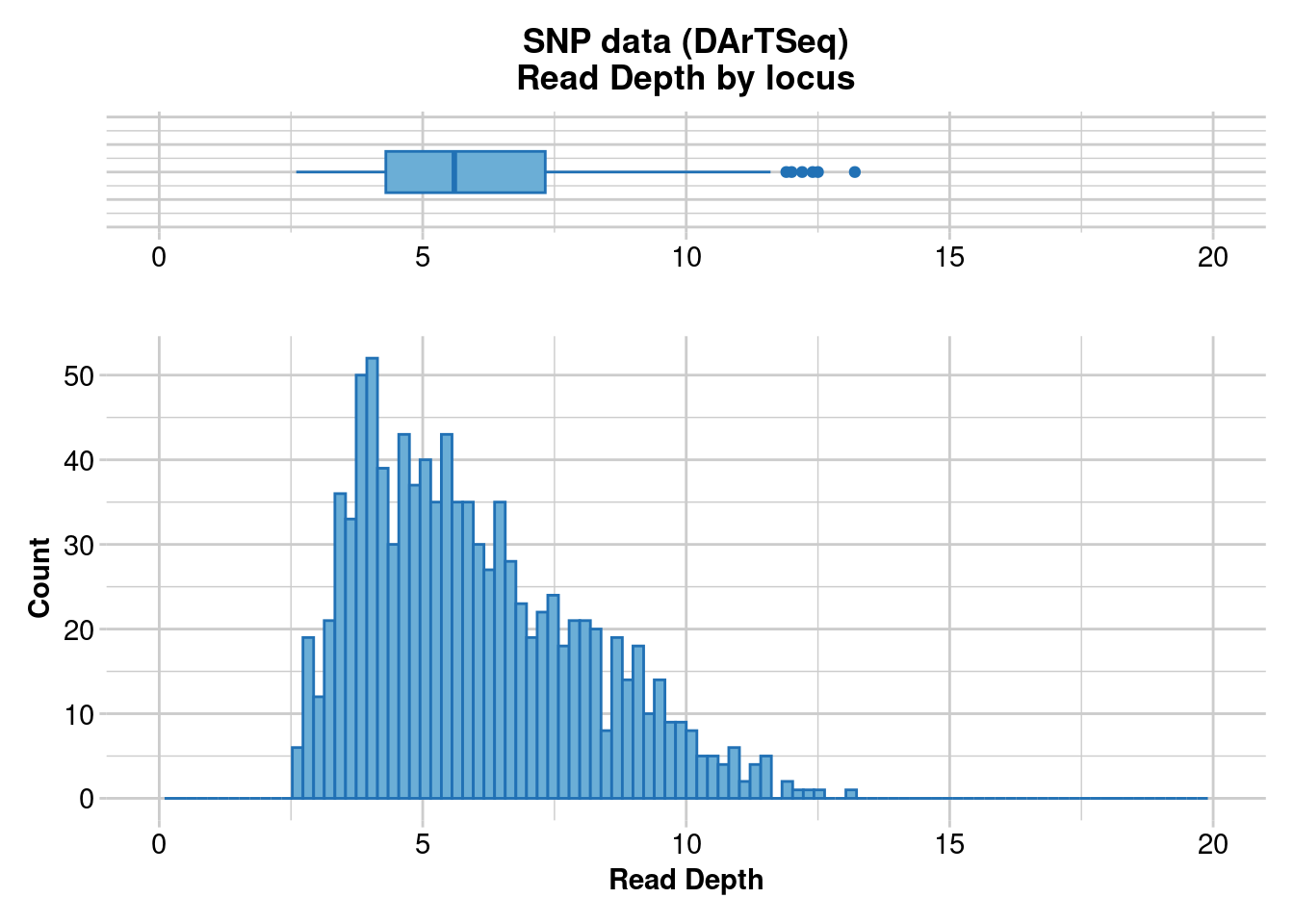

   Quantile Threshold Retained Percent Filtered Percent
1      100%      13.2        1     0.1      999    99.9
2       95%       9.9       51     5.1      949    94.9
3       90%       9.0      105    10.5      895    89.5
4       85%       8.3      151    15.1      849    84.9
5       80%       7.8      208    20.8      792    79.2
6       75%       7.3      258    25.8      742    74.2
7       70%       6.9      304    30.4      696    69.6
8       65%       6.5      354    35.4      646    64.6
9       60%       6.2      404    40.4      596    59.6
10      55%       5.9      451    45.1      549    54.9
11      50%       5.6      504    50.4      496    49.6
12      45%       5.3      563    56.3      437    43.7
13      40%       5.1      602    60.2      398    39.8
14      35%       4.8      659    65.9      341    34.1
15      30%       4.6      702    70.2      298    29.8
16      25%       4.3      752    75.2      248    24.8
17      20%       4.0      823    82.3      177    17.7
18      15%       3.9      852    85.2      148    14.8
19      10%       3.6      906    90.6       94     9.4
20       5%       3.3      956    95.6       44     4.4
21       0%       2.6     1000   100.0        0     0.0
Completed: :: 
 Completed: dartR.base 
 Completed: gl.report.rdepth

EYR.sloppy <- dartR.base::gl.filter.rdepth(EYR, lower = 3, upper = 11, verbose = 0)

# Filter for loci call rate
dartR.base::gl.report.callrate(EYR.sloppy, method = "loc")

Starting :: 
 Starting dartR.base 
 Starting gl.report.callrate 
  Processing genlight object with SNP data
  Reporting Call Rate by Locus
  No. of loci = 958 
  No. of individuals = 782 
    Minimum      :  0.20844 
    1st quartile :  0.7202688 
    Median       :  0.895141 
    Mean         :  0.8131871 
    3r quartile  :  0.950128 
    Maximum      :  0.988491 
    Missing Rate Overall:  0.1868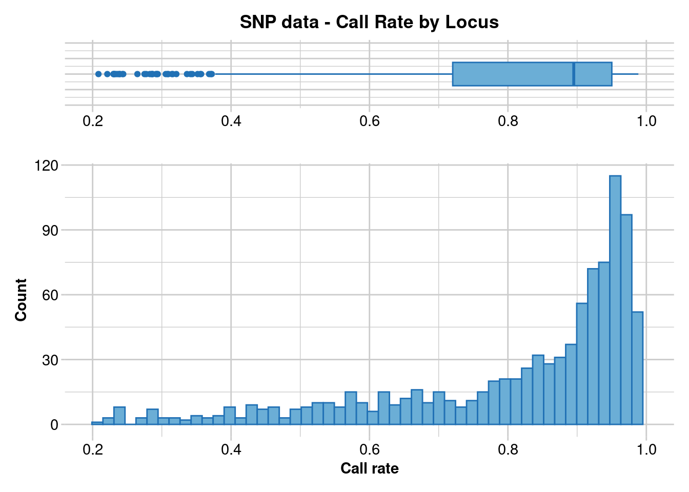

Completed: :: 
 Completed: dartR.base 
 Completed: gl.report.callrate

EYR.sloppy <- dartR.base::gl.filter.callrate(EYR.sloppy, method = "loc",  threshold = 0.75, verbose = 0, recalc = TRUE)

# Filter for individual call rate
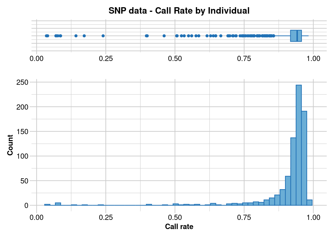
dartR.base::gl.report.callrate(EYR.sloppy, method = "ind")

Starting :: 
 Starting dartR.base 
 Starting gl.report.callrate 
  Processing genlight object with SNP data

  Reporting Call Rate by Individual
  No. of loci = 703 
  No. of individuals = 782 
    Minimum      :  0.03556188 
    1st quartile :  0.9174964 
    Median       :  0.9416785 
    Mean         :  0.9108097 
    3r quartile  :  0.9573257 
    Maximum      :  0.9829303 
    Missing Rate Overall:  0.0892 

Listing 4 populations and their average CallRates
  Monitor again after filtering
  Population CallRate   N
1     Crusoe   0.9027 238
2 Muckleford   0.9073 421
3      Timor   0.9402  52
4     Wombat   0.9371  71

Listing 20 individuals with the lowest CallRates
  Use this list to see which individuals will be lost on filtering by individual
  Set ind.to.list parameter to see more individuals
   Individual   CallRate
1    M18.29.1 0.03556188
2    M18.18.1 0.03982930
3    M18.47.2 0.06970128
4    C18.16.1 0.07112376
5   027-34168 0.07681366
6    C18.15.2 0.08534851
7    C18.21.2 0.08677098
8    M18.47.3 0.14224751
9    M18.35.2 0.17211949
10   M18.20.3 0.24039829
11   M20.70.2 0.39687055
12   C18.28.1 0.39971550
13   C18.17.2 0.46088193
14  027-34065 0.50640114
15   C18.14.1 0.50640114
16   M20.70.3 0.50782361
17  M20.110.1 0.52347084
18   M19.12.1 0.53342817
19    M19.8.1 0.54907539
20   M20.64.3 0.56045519

)

Completed: :: 
 Completed: dartR.base 
 Completed: gl.report.callrate

EYR.sloppy <- dartR.base::gl.filter.callrate(EYR.sloppy, method = "ind", threshold = 0.65, verbose = 0, recalc = TRUE)

# Filter for MAC (= 3)
dartR.base::gl.report.maf(EYR.sloppy)

Starting :: 
 Starting dartR.base 
 Starting gl.report.maf 
  Processing genlight object with SNP data
Starting :: 

 Starting dartR.base 

 Starting gl.report.maf 

  Reporting Minor Allele Frequency (MAF) by Locus for population Crusoe 
  No. of loci = 670 
  No. of individuals = 231 
    Minimum      :  0.0022 
    1st quantile :  0.064825 
    Median       :  0.1582 
    Mean         :  0.1793525 
    3r quantile  :  0.267475 
    Maximum      :  0.4975 
    Missing Rate Overall:  0.08 

  Reporting Minor Allele Frequency (MAF) by Locus for population Muckleford 
  No. of loci = 683 
  No. of individuals = 401 
    Minimum      :  0.0013 
    1st quantile :  0.05875 
    Median       :  0.1404 
    Mean         :  0.172949 
    3r quantile  :  0.2617 
    Maximum      :  0.4985 
    Missing Rate Overall:  0.07 

  Reporting Minor Allele Frequency (MAF) by Locus for population Timor 
  No. of loci = 589 
  No. of individuals = 52 
    Minimum      :  0.0096 
    1st quantile :  0.0673 
    Median       :  0.1667 
    Mean         :  0.1914129 
    3r quantile  :  0.2872 
    Maximum      :  0.5 
    Missing Rate Overall:  0.06 

  Reporting Minor Allele Frequency (MAF) by Locus for population Wombat 
  No. of loci = 627 
  No. of individuals = 71 
    Minimum      :  0.007 
    1st quantile :  0.06385 
    Median       :  0.1449 
    Mean         :  0.1746703 
    3r quantile  :  0.2542 
    Maximum      :  0.5 
    Missing Rate Overall:  0.06 

  Reporting Minor Allele Frequency (MAF) by Locus OVERALL
  No. of loci = 703 
  No. of individuals = 755 
    Minimum      :  3e-04 
    1st quantile :  0.0627 
    Median       :  0.13435 
    Mean         :  0.1696497 
    3r quantile  :  0.246025 
    Maximum      :  0.4991 
    Missing Rate Overall:  0.07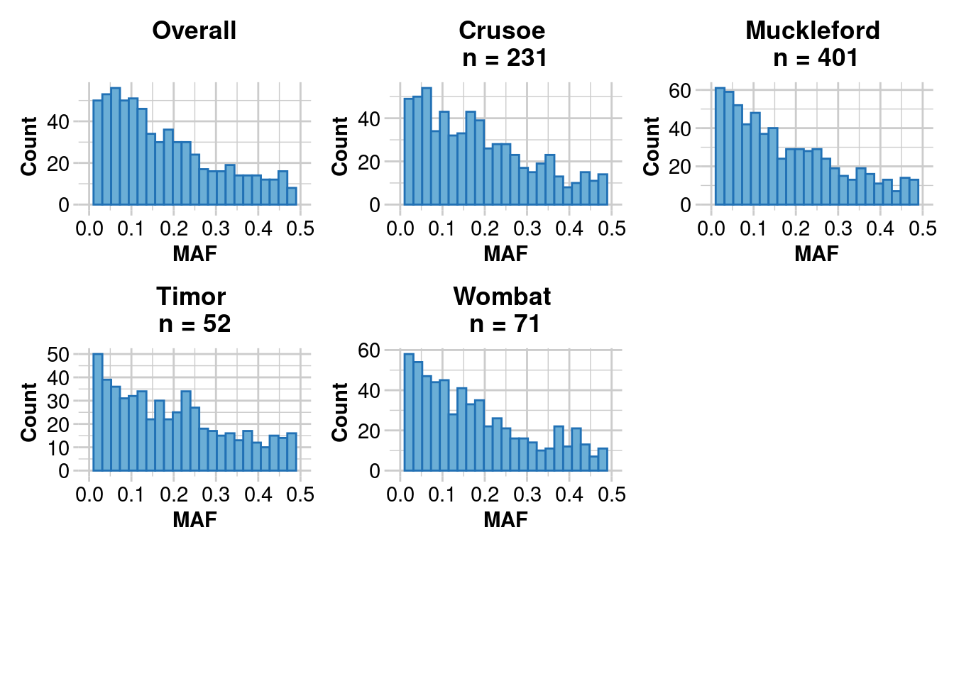

   Quantile Threshold Retained Percent Filtered Percent
1      100%    0.4991        1     0.1      699    99.9
2       95%    0.4343       36     5.1      664    94.9
3       90%    0.3807       71    10.1      629    89.9
4       85%    0.3331      105    15.0      595    85.0
5       80%    0.2858      141    20.1      559    79.9
6       75%    0.2460      176    25.1      524    74.9
7       70%    0.2233      210    30.0      490    70.0
8       65%    0.2003      246    35.1      454    64.9
9       60%    0.1797      280    40.0      420    60.0
10      55%    0.1562      315    45.0      385    55.0
11      50%    0.1341      352    50.3      348    49.7
12      45%    0.1214      386    55.1      314    44.9
13      40%    0.1032      421    60.1      279    39.9
14      35%    0.0904      455    65.0      245    35.0
15      30%    0.0742      490    70.0      210    30.0
16      25%    0.0627      526    75.1      174    24.9
17      20%    0.0476      561    80.1      139    19.9
18      15%    0.0359      595    85.0      105    15.0
19      10%    0.0224      631    90.1       69     9.9
20       5%    0.0059      666    95.1       34     4.9
21       0%    0.0003      700   100.0        0     0.0
Completed: :: 
 Completed: dartR.base 
 Completed: gl.report.maf

EYR.sloppy <- dartR.base::gl.filter.maf(EYR.sloppy, threshold = 3, verbose = 0, recalc = TRUE)

Starting gl.select.colors 
  Warning: Number of required colors not specified, set to 9
  Library: RColorBrewer
  Palette: brewer.pal
  Showing and returning 2 of 9 colors for library RColorBrewer : palette Blues

Completed: gl.select.colors

Filtering SNPs with gl.filter.sexlinked and standard filters (correct)

# Filter for sex-linked loci
correct <- dartR.sexlinked::gl.filter.sexlinked(EYR, system = "zw")  # This is the initial dataset

# We will use correct$autosomal for the next filters

# Filter for read depth
dartR.base::gl.report.rdepth(correct$autosomal)  # This is the filtered dataset

Starting :: 
 Starting dartR.base 
 Starting gl.report.rdepth 
  Processing genlight object with SNP data
  Reporting Read Depth by Locus
  No. of loci = 850 
  No. of individuals = 782 
    Minimum      :  2.6 
    1st quartile :  4.3 
    Median       :  5.6 
    Mean         :  6.008941 
    3r quartile  :  7.4 
    Maximum      :  13.2 
    Missing Rate Overall:  0.18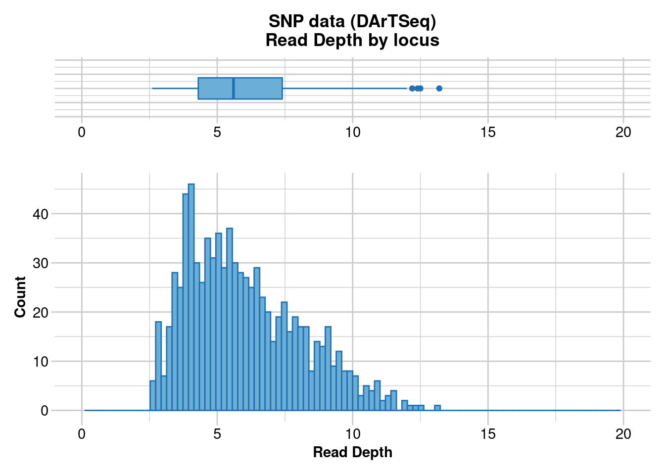

   Quantile Threshold Retained Percent Filtered Percent
1      100%      13.2        1     0.1      849    99.9
2       95%       9.9       45     5.3      805    94.7
3       90%       9.1       88    10.4      762    89.6
4       85%       8.4      129    15.2      721    84.8
5       80%       7.9      173    20.4      677    79.6
6       75%       7.4      220    25.9      630    74.1
7       70%       6.9      264    31.1      586    68.9
8       65%       6.5      305    35.9      545    64.1
9       60%       6.2      350    41.2      500    58.8
10      55%       5.9      391    46.0      459    54.0
11      50%       5.6      435    51.2      415    48.8
12      45%       5.4      472    55.5      378    44.5
13      40%       5.1      519    61.1      331    38.9
14      35%       4.9      555    65.3      295    34.7
15      30%       4.6      603    70.9      247    29.1
16      25%       4.3      645    75.9      205    24.1
17      20%       4.0      705    82.9      145    17.1
18      15%       3.9      730    85.9      120    14.1
19      10%       3.6      774    91.1       76     8.9
20       5%       3.3      812    95.5       38     4.5
21       0%       2.6      850   100.0        0     0.0
Completed: :: 
 Completed: dartR.base 
 Completed: gl.report.rdepth

EYR.correct <- dartR.base::gl.filter.rdepth(correct$autosomal, lower = 3, upper = 11, verbose = 0)

# Filter for loci call rate
dartR.base::gl.report.callrate(EYR.correct, method = "loc")

Starting :: 
 Starting dartR.base 
 Starting gl.report.callrate 
  Processing genlight object with SNP data
  Reporting Call Rate by Locus
  No. of loci = 811 
  No. of individuals = 782 
    Minimum      :  0.20844 
    1st quartile :  0.7436065 
    Median       :  0.900256 
    Mean         :  0.8192658 
    3r quartile  :  0.951407 
    Maximum      :  0.988491 
    Missing Rate Overall:  0.1807

Completed: :: 
 Completed: dartR.base 
 Completed: gl.report.callrate

EYR.correct <- dartR.base::gl.filter.callrate(EYR.correct, method = "loc",  threshold = 0.75, verbose = 0, recalc = TRUE)

# Filter for individual call rate
dartR.base::gl.report.callrate(EYR.correct, method = "ind")

Starting :: 
 Starting dartR.base 
 Starting gl.report.callrate 
  Processing genlight object with SNP data

  Reporting Call Rate by Individual
  No. of loci = 605 
  No. of individuals = 782 
    Minimum      :  0.03801653 
    1st quartile :  0.9173554 
    Median       :  0.9438017 
    Mean         :  0.9120479 
    3r quartile  :  0.9586777 
    Maximum      :  0.9818182 
    Missing Rate Overall:  0.088 

Listing 4 populations and their average CallRates
  Monitor again after filtering
  Population CallRate   N
1     Crusoe   0.9037 238
2 Muckleford   0.9090 421
3      Timor   0.9418  52
4     Wombat   0.9365  71

Listing 20 individuals with the lowest CallRates
  Use this list to see which individuals will be lost on filtering by individual
  Set ind.to.list parameter to see more individuals
   Individual   CallRate
1    M18.29.1 0.03801653
2    M18.18.1 0.04462810
3    M18.47.2 0.06776860
4    C18.16.1 0.07438017
5   027-34168 0.08760331
6    C18.15.2 0.08760331
7    C18.21.2 0.08760331
8    M18.47.3 0.13719008
9    M18.35.2 0.18016529
10   M18.20.3 0.24132231
11   C18.28.1 0.41487603
12   M20.70.2 0.42644628
13   C18.17.2 0.44628099
14  027-34065 0.49586777
15   C18.14.1 0.49752066
16  M20.110.1 0.53057851
17   M20.70.3 0.53553719
18   M19.12.1 0.54380165
19    M19.8.1 0.56694215
20   M19.33.2 0.57851240

)

Completed: :: 
 Completed: dartR.base 
 Completed: gl.report.callrate

EYR.correct <- dartR.base::gl.filter.callrate(EYR.correct, method = "ind", threshold = 0.65, verbose = 0, recalc = TRUE)

# Filter for MAC (= 3)
dartR.base::gl.report.maf(EYR.correct)

Starting :: 
 Starting dartR.base 
 Starting gl.report.maf 
  Processing genlight object with SNP data
Starting :: 

 Starting dartR.base 

 Starting gl.report.maf 

  Reporting Minor Allele Frequency (MAF) by Locus for population Crusoe 
  No. of loci = 573 
  No. of individuals = 231 
    Minimum      :  0.0022 
    1st quantile :  0.06 
    Median       :  0.1488 
    Mean         :  0.1741178 
    3r quantile  :  0.2646 
    Maximum      :  0.4975 
    Missing Rate Overall:  0.08 

  Reporting Minor Allele Frequency (MAF) by Locus for population Muckleford 
  No. of loci = 585 
  No. of individuals = 401 
    Minimum      :  0.0013 
    1st quantile :  0.055 
    Median       :  0.129 
    Mean         :  0.163993 
    3r quantile  :  0.2474 
    Maximum      :  0.4985 
    Missing Rate Overall:  0.07 

  Reporting Minor Allele Frequency (MAF) by Locus for population Timor 
  No. of loci = 504 
  No. of individuals = 52 
    Minimum      :  0.0096 
    1st quantile :  0.068275 
    Median       :  0.1635 
    Mean         :  0.1898613 
    3r quantile  :  0.286075 
    Maximum      :  0.5 
    Missing Rate Overall:  0.06 

  Reporting Minor Allele Frequency (MAF) by Locus for population Wombat 
  No. of loci = 536 
  No. of individuals = 71 
    Minimum      :  0.007 
    1st quantile :  0.062475 
    Median       :  0.13805 
    Mean         :  0.1706063 
    3r quantile  :  0.2509 
    Maximum      :  0.5 
    Missing Rate Overall:  0.06 

  Reporting Minor Allele Frequency (MAF) by Locus OVERALL
  No. of loci = 605 
  No. of individuals = 755 
    Minimum      :  3e-04 
    1st quantile :  0.058025 
    Median       :  0.1306 
    Mean         :  0.1628656 
    3r quantile  :  0.23785 
    Maximum      :  0.4991 
    Missing Rate Overall:  0.07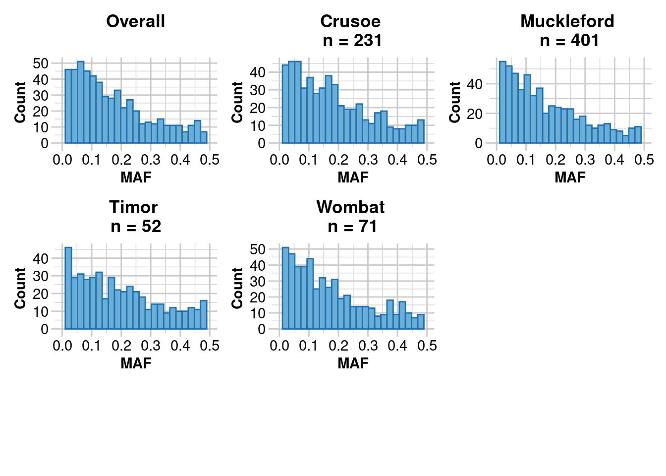

   Quantile Threshold Retained Percent Filtered Percent
1      100%    0.4991        1     0.2      601    99.8
2       95%    0.4367       31     5.1      571    94.9
3       90%    0.3771       61    10.1      541    89.9
4       85%    0.3250       91    15.1      511    84.9
5       80%    0.2747      121    20.1      481    79.9
6       75%    0.2387      151    25.1      451    74.9
7       70%    0.2132      181    30.1      421    69.9
8       65%    0.1916      211    35.0      391    65.0
9       60%    0.1720      241    40.0      361    60.0
10      55%    0.1486      271    45.0      331    55.0
11      50%    0.1306      302    50.2      300    49.8
12      45%    0.1118      332    55.1      270    44.9
13      40%    0.0975      362    60.1      240    39.9
14      35%    0.0808      392    65.1      210    34.9
15      30%    0.0700      422    70.1      180    29.9
16      25%    0.0578      452    75.1      150    24.9
17      20%    0.0445      482    80.1      120    19.9
18      15%    0.0300      512    85.0       90    15.0
19      10%    0.0174      542    90.0       60    10.0
20       5%    0.0046      572    95.0       30     5.0
21       0%    0.0003      602   100.0        0     0.0
Completed: :: 
 Completed: dartR.base 
 Completed: gl.report.maf

EYR.correct <- dartR.base::gl.filter.maf(EYR.correct, threshold = 3, verbose = 0, recalc = TRUE)

Starting gl.select.colors 
  Warning: Number of required colors not specified, set to 9
  Library: RColorBrewer
  Palette: brewer.pal
  Showing and returning 2 of 9 colors for library RColorBrewer : palette Blues

Completed: gl.select.colors

3. Changes in PCA before and after removing the SLM?

PCA on sloppy dataset (only standard filters)

PCA.sloppy <- dartR.base::gl.pcoa(EYR.sloppy, verbose = 0)
dartR.base::gl.pcoa.plot(PCA.sloppy, EYR.sloppy, xaxis = 1, yaxis = 2)
dartR.base::gl.pcoa.plot(PCA.sloppy, EYR.sloppy, xaxis = 2, yaxis = 3)

Starting gl.colors 
Selected color type 2 
Completed: gl.colors 
Starting :: 
 Starting dartR.base 
 Starting gl.pcoa.plot 
  Processing an ordination file (glPca)
  Processing genlight object with SNP data
Package directlabels  needed for this function to work. Please install it.
[1] -1
Starting :: 
 Starting dartR.base 
 Starting gl.pcoa.plot 
  Processing an ordination file (glPca)
  Processing genlight object with SNP data
Package directlabels  needed for this function to work. Please install it.
[1] -1

PCA on correct dataset (gl.filter.sexlinked and standard filters)

PCA.correct <- dartR.base::gl.pcoa(EYR.correct, verbose = 0)
dartR.base::gl.pcoa.plot(PCA.correct, EYR.correct, xaxis = 1, yaxis = 2)
dartR.base::gl.pcoa.plot(PCA.correct, EYR.correct, xaxis = 2, yaxis = 3)

Starting gl.colors 
Selected color type 2 
Completed: gl.colors 
Starting :: 
 Starting dartR.base 
 Starting gl.pcoa.plot 
  Processing an ordination file (glPca)
  Processing genlight object with SNP data
Package directlabels  needed for this function to work. Please install it.
[1] -1
Starting :: 
 Starting dartR.base 
 Starting gl.pcoa.plot 
  Processing an ordination file (glPca)
  Processing genlight object with SNP data
Package directlabels  needed for this function to work. Please install it.
[1] -1

4. Differences in genetic diversity and fixation indices between autosomal and SLM?

# Basic stats
basic.sloppy  <- dartR.base::utils.basic.stats(EYR.sloppy)
basic.correct <- dartR.base::utils.basic.stats(EYR.correct)
basic.sloppy$overall

     Ho      Hs      Ht     Dst     Htp    Dstp     Fst    Fstp     Fis    Dest 
 0.1603  0.2376  0.2464  0.0087  0.2487  0.0148  0.0355  0.0596  0.3256  0.0259 
Gst_max   Gst_H 
 0.7141  0.0834

basic.correct$overall

     Ho      Hs      Ht     Dst     Htp    Dstp     Fst    Fstp     Fis    Dest 
 0.1579  0.2302  0.2375  0.0073  0.2398  0.0128  0.0307  0.0532  0.3139  0.0221 
Gst_max   Gst_H 
 0.7229  0.0737

# Genetic diversity per pop
divers.sloppy <- dartR.base::gl.report.diversity(EYR.sloppy, pbar = FALSE, table = FALSE, verbose = 0)

  Processing genlight object with SNP data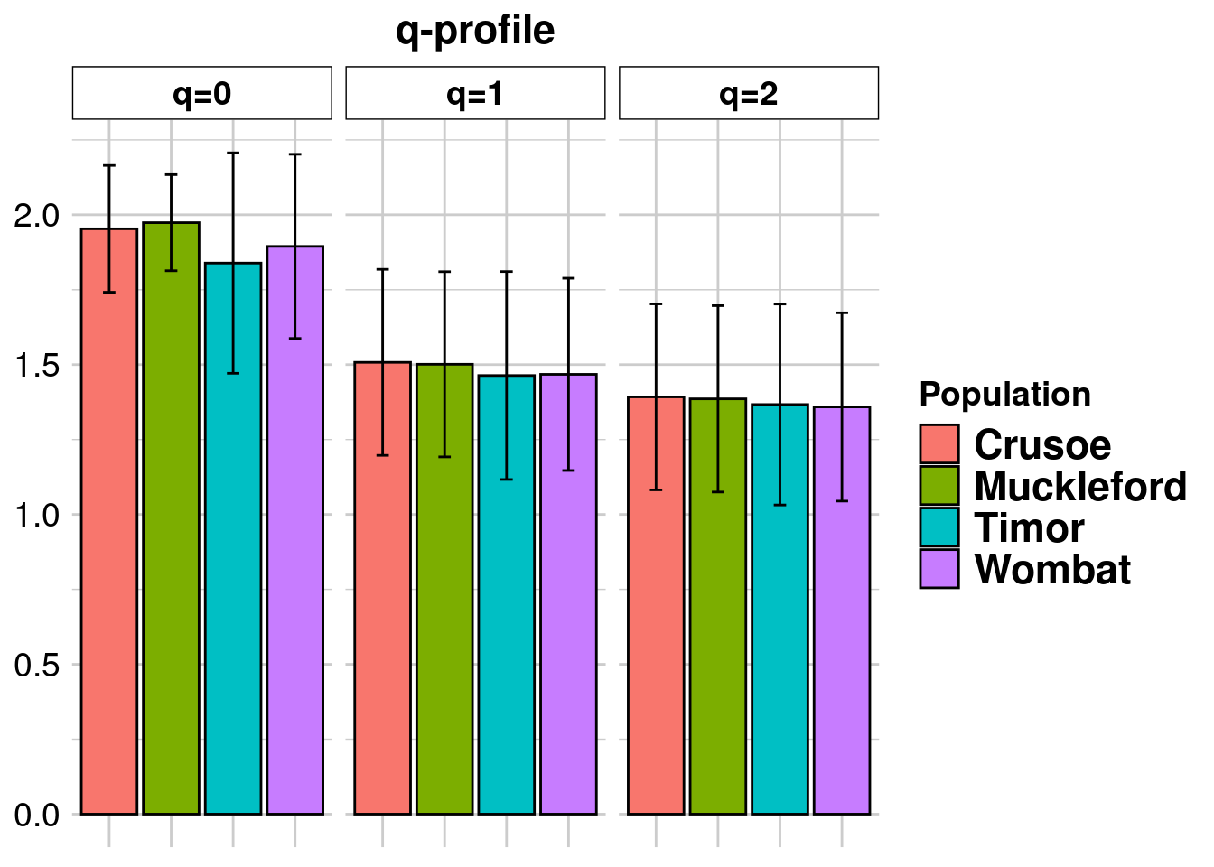

divers.correct <- dartR.base::gl.report.diversity(EYR.correct, pbar = FALSE, table = FALSE, verbose = 0)

  Processing genlight object with SNP data

divers.sloppy$one_H_alpha

    Crusoe Muckleford      Timor     Wombat 
 0.3884366  0.3844244  0.3519361  0.3591638

divers.correct$one_H_alpha

    Crusoe Muckleford      Timor     Wombat 
 0.3766483  0.3689045  0.3468530  0.3503540

divers.sloppy$one_H_beta

                Crusoe Muckleford      Timor     Wombat
Crusoe              NA 0.02660219 0.09367676 0.06237102
Muckleford 0.006274769         NA 0.07326488 0.06577359
Timor      0.022518949 0.02452504         NA 0.08763552
Wombat     0.018905085 0.02091118 0.03715536         NA

divers.correct$one_H_beta

                Crusoe Muckleford      Timor     Wombat
Crusoe              NA 0.02545762 0.08568969 0.05988791
Muckleford 0.005778848         NA 0.06967786 0.06243346
Timor      0.016804630 0.02067653         NA 0.08306746
Wombat     0.015054123 0.01892602 0.02995180         NA

# Fixation indices
dartR.base::gl.fst.pop(EYR.sloppy, verbose = 0)

               Crusoe Muckleford      Timor Wombat
Crusoe             NA         NA         NA     NA
Muckleford 0.03160198         NA         NA     NA
Timor      0.04023766 0.05408752         NA     NA
Wombat     0.05466955 0.02407235 0.08452847     NA

dartR.base::gl.fst.pop(EYR.correct, verbose = 0)

               Crusoe Muckleford      Timor Wombat
Crusoe             NA         NA         NA     NA
Muckleford 0.02777612         NA         NA     NA
Timor      0.04008148 0.04786375         NA     NA
Wombat     0.04413257 0.02208816 0.07111737     NA

dartR.base::gl.report.fstat(EYR.sloppy, verbose = 0)

Starting gl.colors 
Selected color type div 
Completed: gl.colors

$Stat_matrices
$Stat_matrices$Fst
           Crusoe Muckleford  Timor Wombat
Crusoe         NA     0.0148 0.0171 0.0255
Muckleford 0.0148         NA 0.0249 0.0096
Timor      0.0171     0.0249     NA 0.0387
Wombat     0.0255     0.0096 0.0387     NA

$Stat_matrices$Fstp
           Crusoe Muckleford  Timor Wombat
Crusoe         NA     0.0356 0.0545 0.0669
Muckleford 0.0356         NA 0.0681 0.0337
Timor      0.0545     0.0681     NA 0.1046
Wombat     0.0669     0.0337 0.1046     NA

$Stat_matrices$Dest
           Crusoe Muckleford  Timor Wombat
Crusoe         NA     0.0236 0.0351 0.0434
Muckleford 0.0236         NA 0.0437 0.0213
Timor      0.0351     0.0437     NA 0.0657
Wombat     0.0434     0.0213 0.0657     NA

$Stat_matrices$Gst_H
           Crusoe Muckleford  Timor Wombat
Crusoe         NA     0.0566 0.0850 0.1047
Muckleford 0.0566         NA 0.1059 0.0525
Timor      0.0850     0.1059     NA 0.1603
Wombat     0.1047     0.0525 0.1603     NA


[[2]]
      Stat_tables.Crusoe_vs_Muckleford Stat_tables.Crusoe_vs_Timor
Fst                             0.0148                      0.0171
Fstp                            0.0356                      0.0545
Dest                            0.0236                      0.0351
Gst_H                           0.0566                      0.0850
      Stat_tables.Crusoe_vs_Wombat Stat_tables.Muckleford_vs_Timor
Fst                         0.0255                          0.0249
Fstp                        0.0669                          0.0681
Dest                        0.0434                          0.0437
Gst_H                       0.1047                          0.1059
      Stat_tables.Muckleford_vs_Wombat Stat_tables.Timor_vs_Wombat
Fst                             0.0096                      0.0387
Fstp                            0.0337                      0.1046
Dest                            0.0213                      0.0657
Gst_H                           0.0525                      0.1603

dartR.base::gl.report.fstat(EYR.correct, verbose = 0)

Starting gl.colors 
Selected color type div 
Completed: gl.colors

$Stat_matrices
$Stat_matrices$Fst
           Crusoe Muckleford  Timor Wombat
Crusoe         NA     0.0128 0.0168 0.0199
Muckleford 0.0128         NA 0.0212 0.0085
Timor      0.0168     0.0212     NA 0.0313
Wombat     0.0199     0.0085 0.0313     NA

$Stat_matrices$Fstp
           Crusoe Muckleford  Timor Wombat
Crusoe         NA     0.0317 0.0540 0.0556
Muckleford 0.0317         NA 0.0608 0.0315
Timor      0.0540     0.0608     NA 0.0903
Wombat     0.0556     0.0315 0.0903     NA

$Stat_matrices$Dest
           Crusoe Muckleford  Timor Wombat
Crusoe         NA     0.0199 0.0337 0.0344
Muckleford 0.0199         NA 0.0373 0.0189
Timor      0.0337     0.0373     NA 0.0547
Wombat     0.0344     0.0189 0.0547     NA

$Stat_matrices$Gst_H
           Crusoe Muckleford  Timor Wombat
Crusoe         NA     0.0492 0.0832 0.0856
Muckleford 0.0492         NA 0.0930 0.0480
Timor      0.0832     0.0930     NA 0.1368
Wombat     0.0856     0.0480 0.1368     NA


[[2]]
      Stat_tables.Crusoe_vs_Muckleford Stat_tables.Crusoe_vs_Timor
Fst                             0.0128                      0.0168
Fstp                            0.0317                      0.0540
Dest                            0.0199                      0.0337
Gst_H                           0.0492                      0.0832
      Stat_tables.Crusoe_vs_Wombat Stat_tables.Muckleford_vs_Timor
Fst                         0.0199                          0.0212
Fstp                        0.0556                          0.0608
Dest                        0.0344                          0.0373
Gst_H                       0.0856                          0.0930
      Stat_tables.Muckleford_vs_Wombat Stat_tables.Timor_vs_Wombat
Fst                             0.0085                      0.0313
Fstp                            0.0315                      0.0903
Dest                            0.0189                      0.0547
Gst_H                           0.0480                      0.1368

Exercise data 3 - Bull shark

Data from Devloo‐Delva et al. (2023).

Load data

print(load("data/Bull_shark_DArTseq_genlight_for_sex-linked_markers.Rdata"))

[1] "data.gl"

data.gl@n.loc

[1] 93202

table(data.gl@pop)


E-ATL  E-IO  Fiji Japan  N-IO W-ATL  W-IO W-PAC 
    2    36     8    14    20    36    40    26

table(data.gl@other$ind.metrics$pop)


E-ATL  E-IO  Fiji Japan  N-IO W-ATL  W-IO W-PAC 
    2    36     8    14    20    36    40    26

table(data.gl@other$ind.metrics$sex, useNA = "ifany")


   F    M <NA> 
  85   64   33

1. Number of sex-linked markers?

ncores <- min(4, parallel::detectCores())
#still takes some minutes to run
res <- dartR.sexlinked::gl.filter.sexlinked(gl = data.gl, system = "xy", plots = TRUE, ncores = ncores)

Detected 85 females and 64 males.

Starting phase 1. Working in parallel...

Building call rate plots.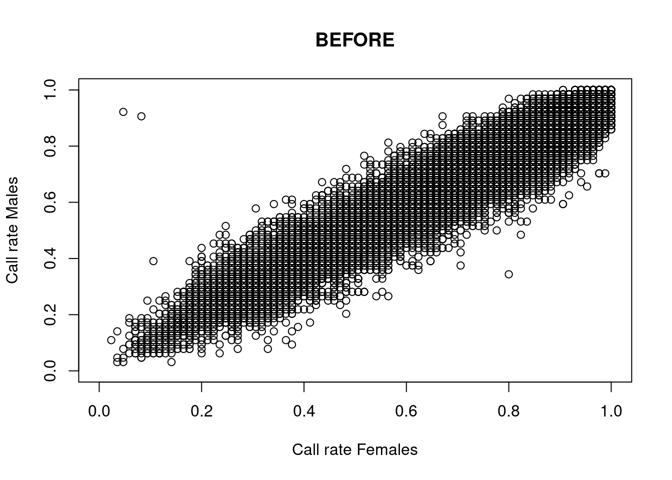

Done. Starting phase 2.

Building heterozygosity plots.

Done building heterozygosity plots.

**FINISHED** Total of analyzed loci: 93202.
Found 9 sex-linked loci:
   2 Y-linked loci
   2 sex-biased loci
   4 X-linked loci
   1 XY gametologs.
And 93193 autosomal loci.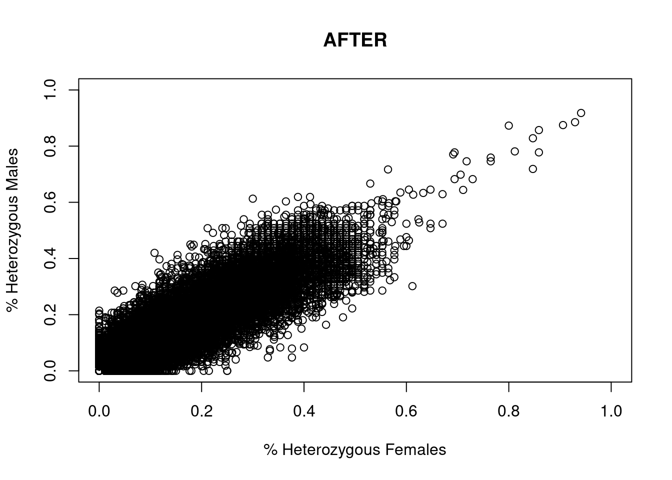

2. Individuals with wrong sexID?

#check if you can increase the number of cores
sexID <- dartR.sexlinked::gl.infer.sex(gl_sex_filtered = res, system = "xy", seed = 124)

Not enough gametologs (need at least 5). Assigning NA...

***FINISHED***

knitr::kable(head(sexID))

agreed.sex <- sub(pattern = "\\*", replacement = "", x = sexID$agreed.sex) # remove asterisk
sum(data.gl$other$ind.metrics$sex != agreed.sex, na.rm = TRUE)

	id	y.linked.sex	#called	#missing	x.linked.sex	#Het.x	#Hom.x	gametolog.sex	#Het.g	#Hom.g	agreed.sex
CL-FIJ002-F	CL-FIJ002-F	F	0	2	F	4	0	NA	NA	NA	F
CL-FIJ003-M	CL-FIJ003-M	M	2	0	M	0	4	NA	NA	NA	M
CL-FIJ008-F	CL-FIJ008-F	F	0	2	F	2	2	NA	NA	NA	F
CL-FIJ010-F	CL-FIJ010-F	F	0	2	F	3	1	NA	NA	NA	F
CL-FIJ015-F	CL-FIJ015-F	F	0	2	F	4	0	NA	NA	NA	F
CL-FIJ018-F	CL-FIJ018-F	F	0	2	F	3	1	NA	NA	NA	F

[1] 8

Exercise data 4 - Blue shark

Data from Nikolic et al. (2023).

Load data

print(load("data/Blue_shark_DArTseq_genlight_for_sex-linked_markers.Rdata"))

[1] "data.gl"

data.gl@n.loc

[1] 172384

table(data.gl@pop)


   EIO   MED1   MED2   NATL  NEATL    NIO   NPAC   SAF1   SAF2 SWPAC1 SWPAC2 
     8     34     20     49     26     27      4     21     89     30     16 
SWPAC3    WIO 
    11     29

table(data.gl@other$ind.metrics$pop)


   EIO   MED1   MED2   NATL  NEATL    NIO   NPAC   SAF1   SAF2 SWPAC1 SWPAC2 
     8     34     20     49     26     27      4     21     89     30     16 
SWPAC3    WIO 
    11     29

table(data.gl@other$ind.metrics$sex, useNA = "ifany")


   F    M <NA> 
 104  111  149

1. Number of sex-linked markers?

#check if you can increase the number of cores
# ncores <- min(4,parallel::detectCores())
# resbull <- dartR.sexlinked::gl.filter.sexlinked(gl = data.gl, system = "xy", plots = TRUE, ncores = ncores)
#load results from previous run
resbull <- readRDS("./data/resbull.rds")

2. Individuals with wrong sexID?

#check if you can increase the number of cores
sexID <- dartR.sexlinked::gl.infer.sex(gl_sex_filtered = resbull, system = "xy", seed = 124)

Not enough gametologs (need at least 5). Assigning NA...

***FINISHED***

knitr::kable(head(sexID))

agreed.sex <- sub(pattern = "\\*", replacement = "", x = sexID$agreed.sex) # remove asterisk
sum(data.gl$other$ind.metrics$sex != agreed.sex, na.rm = TRUE)

	id	y.linked.sex	#called	x.linked.sex	#Het.x	#Hom.x	gametolog.sex	#Het.g	#Hom.g	agreed.sex
60088	60088	M	2	M	0	22	NA	NA	NA	M
60160	60160	M	2	M	0	21	NA	NA	NA	M
60168	60168	M	2	M	0	22	NA	NA	NA	M
60176	60176	M	2	M	0	21	NA	NA	NA	M
60096	60096	M	2	M	0	22	NA	NA	NA	M
60104	60104	M	2	M	1	19	NA	NA	NA	M

[1] 22

Required packages

Dataset 1 - ZW//ZZ - The Yellow Tufted Honeyeater

Load data

Run gl.filter.sexlinked

Run gl.infer.sex

Dataset 2 - XX/XY - The Leadbeater’s possum

Load data

Run gl.filter.sexlinked

Run gl.infer.sex

EXERCISE

Further study

Exercise data 1 - Your own data

Exercise data 2 - The Eastern Yellow Robin

Load data

1. Number of sex-linked markers?

2. Individuals with wrong sexID?

Processing SNPs with two filtering regimes

Filtering SNPs only with standard filters (sloppy)

Filtering SNPs with gl.filter.sexlinked and standard filters (correct)

3. Changes in PCA before and after removing the SLM?

PCA on sloppy dataset (only standard filters)

PCA on correct dataset (gl.filter.sexlinked and standard filters)

4. Differences in genetic diversity and fixation indices between autosomal and SLM?

Exercise data 3 - Bull shark

Load data

1. Number of sex-linked markers?

2. Individuals with wrong sexID?

Exercise data 4 - Blue shark

Load data

1. Number of sex-linked markers?

2. Individuals with wrong sexID?

Run `gl.filter.sexlinked`

Run `gl.infer.sex`

Run `gl.filter.sexlinked`

Run `gl.infer.sex`