2  Pop Gen In Conservation

Session Presenters

Required packages

#BiocManager::install("LEA")
#devtools::install_github("tdhock/directlabels")

library(dartRverse)

library(ggplot2)
library(data.table)

library(leaflet.minicharts)
library(LEA)

make sure you have the packages installed, see Install dartRverse

Introduction

Here is an introductory video on genetic diversity measures that is assumed knowledge for this session.

For more details see Sherwin et al. (2017).

Exercise

Task

You have been asked to evaluate the ‘genetic health’ of a population at a restoration site, which has been established two years earlier as a results of the drying of a wet land due to urban development. The corporate responsible for the restoration project claims that the area can now sustain a high density population of the species A, which previously only occurred in the forested areas west and east of the previously existing wet land. Species A is a long lived terrestrial animal.

Compute genetic diversity metrics (e.g. \(He\), \(Ho\), \(Fis\)) with the data generated by the 100 samples collected and provide a recommendation on whether the restoration project was successful and whether the studied population is likely to required continued active management in the short term.

Load data

# Load the data
glsim <- gl.load("./data/sess2_glsim.rds")

#check the population size and number of populations
table(pop(glsim))

popA 
 100 

#number of loci
nLoc(glsim)

[1] 2500

Different dynamics, same result

Several descriptive genetic parameters are almost routinely computed, and one would be tempted to interpret them with a standardised approach. For example, low genetic diversity is often considered as an indication that the population size is small. If the inbreeding coefficient (\(Fis\)) is positive, that is often taken as an indication that the population is inbred and potentially at risk of inbreeding depression. However, there are situation where different dynamics can produce the same result. It is not always easy to diagnose these situations and identify the cause of our results, but my recommendation would be to give priority to your understanding of the biology, ecology and history of the populations and species you are working with. If the suggested interpretation do not fit your understanding of the ecology or demographics of the populations you are working with, explore possible alternative explanations. In the example above, a low genetic diversity can also occur because of a severe bottleneck even if the population has then recovered to large numbers.

Recall that \(Fis = (He-Ho)/He\), hence any cause of alteration of HWE can cause an increased/decrease \(Fis\) as well sampling effects. For example, the selective sampling of related individuals (e.g. when sampling individuals within family groups - as often happens with feral pigs/boar - or when you are sampling intensively within the dispersal distance range of few individuals) can cause your samples not to be representative of the population, and while your analysis could indicate inbreeding, this may not be the case at population level. Wahlund effect is also another common cause of increased \(Fis\).

Let’s have a look at an example of what happens if our sampling design caused us to sample selectively related individuals. We are going to use a simulated dataset based on the concept presented in Pacioni et al (2020) where females intensively trapped (using a grid design, ‘G’) within an area that didn’t encompassed multiple home ranges were highly related. ON the contrary, individuals trapped along transect (‘T’) that extended over multiple home ranges were an actual random rapresentation of the population.

Load data

glw <- gl.load("./data/sess2_glDes.rds")
#check the population size and number of populations
table(pop(glw)) # G stands for trapped in a grid, T for transect
#number of loci
nLoc(glw)

glw <- gl.filter.monomorphs(glw, verbose = 5)

Calculate Relatedness

# Run EMIBD9 to detect related individuals. Output saved to save time
#ibd9 <- gl.run.EMIBD9(glw, Inbreed = FALSE, 
 #                     emibd9.path = "E:/Software/Genetic software/EMIBD9")
#saveRDS(ibd9, file="Gen Diversity/ibd9.rds")

# Load EMIBD9 results
ibd9 <- readRDS("./data/sess2_ibd9.rds")

# Do some manipulation to have everything in one table
ibd9Tab <- ibd9[[2]]
# Kick out self comparisons
ibd9Tab <- ibd9Tab[ibd9Tab$Indiv1 != ibd9Tab$Indiv2,  c(1, 2, 21)]
# Add trapping des for each individuals
Des1 <- pop(glw)[as.numeric(ibd9Tab$Indiv1)]
Des2 <- pop(glw)[as.numeric(ibd9Tab$Indiv2)]
# Flag pairs trapping within G, T and in between (BW)
PDes <- ifelse((Des1 == "G" & Des2 == "G"), yes = "G", 
       no = ifelse((Des1 == "T" & Des2 == "T"), yes = "T", "BW"))
# Combine together
ibd9DT <- data.table(cbind(ibd9Tab, Des1, Des2, PDes))
# Compute the mean relatedness
ibd9DT[, mean(as.numeric(`r(1,2)`)), by=PDes]

     PDes         V1
   <char>      <num>
1:      T 0.03800294
2:     BW 0.01454867
3:      G 0.08464706

Relatedness results

Mean relatedness for animals trapped in the grid is 3 times those trapped with a transect. There are also a series of other interesting things that happens: Mean relatedness of animals trapped in the grid is just marginally above the mean expected for first cousins (~0.06). However, more than half of the comparisons were between half sibs or more related individuals:

ibd9DT[, sum(`r(1,2)`>=0.125), by=PDes] # HS or more

     PDes    V1
   <char> <int>
1:      T     0
2:     BW     0
3:      G   512

ibd9DT[, sum(`r(1,2)`>=0.25), by=PDes] # FS or PO

     PDes    V1
   <char> <int>
1:      T     0
2:     BW     0
3:      G    92

# Recall that the number of pairwise comparisons within 'G' is
nG <- sum(pop(glw) == "G")
nG*(nG-1)/2

[1] 1770

Only a limited number of loci are out of HWE after correction for multiple comparisons

hwe <- gl.report.hwe(glw, multi_comp = TRUE)

Starting gl.report.hwe 
  Processing genlight object with SNP data
Package HardyWeinberg  needed for this function to work. Please install it.

But incredibly, because of the het excess, \(Fis\) in ‘G’ is negative suggesting a outbred population!

het <- gl.report.heterozygosity(glw)

Starting gl.report.heterozygosity 
  Processing genlight object with SNP data
  Calculating Observed Heterozygosities, averaged across
                    loci, for each population
  Calculating Expected Heterozygosities

Starting gl.colors 
Selected color type dis 
Completed: gl.colors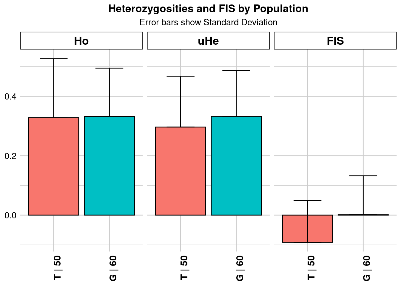 

  pop n.Ind n.Loc n.Loc.adj polyLoc monoLoc all_NALoc       Ho     HoSD
T   T    50   992         1     982      10         0 0.332258 0.162559
G   G    60   992         1     959      33         0 0.327991 0.198620
      HoSE HoLCI HoHCI   Ho.adj Ho.adjSD Ho.adjSE Ho.adjLCI Ho.adjHCI       He
T 0.005161    NA    NA 0.332258 0.162559 0.005161        NA        NA 0.329298
G 0.006306    NA    NA 0.327991 0.198620 0.006306        NA        NA 0.294170
      HeSD     HeSE HeLCI HeHCI      uHe    uHeSD    uHeSE uHeLCI uHeHCI
T 0.152419 0.004839    NA    NA 0.332624 0.153958 0.004888     NA     NA
G 0.169669 0.005387    NA    NA 0.296642 0.171094 0.005432     NA     NA
    He.adj He.adjSD He.adjSE He.adjLCI He.adjHCI       FIS    FISSD    FISSE
T 0.329298 0.152419 0.004839        NA        NA  0.001446 0.130990 0.004159
G 0.294170 0.169669 0.005387        NA        NA -0.091603 0.140922 0.004474
  FISLCI FISHCI
T     NA     NA
G     NA     NA
Completed: gl.report.heterozygosity 

Interpreting results

In our task, when the restoration project took place, two separate populations came in contact, creating an admixture zone. As the species is long-lived there has not been enough mixing and turnover for the two amalgamate. The lack of HWE and increased \(Fis\) is a result of the Wahlund effect.

Exercise data

gl.report.heterozygosity(glsim)

Starting gl.report.heterozygosity 
  Processing genlight object with SNP data
  Calculating Observed Heterozygosities, averaged across
                    loci, for each population
  Calculating Expected Heterozygosities

Starting gl.colors 
Selected color type dis 
Completed: gl.colors 

      pop n.Ind n.Loc n.Loc.adj polyLoc monoLoc all_NALoc       Ho     HoSD
popA popA   100  2500         1    2500       0         0 0.386004 0.142553
         HoSE HoLCI HoHCI   Ho.adj Ho.adjSD Ho.adjSE Ho.adjLCI Ho.adjHCI
popA 0.002851    NA    NA 0.386004 0.142553 0.002851        NA        NA
           He     HeSD     HeSE HeLCI HeHCI      uHe   uHeSD    uHeSE uHeLCI
popA 0.441149 0.096207 0.001924    NA    NA 0.443366 0.09669 0.001934     NA
     uHeHCI   He.adj He.adjSD He.adjSE He.adjLCI He.adjHCI      FIS    FISSD
popA     NA 0.441149 0.096207 0.001924        NA        NA 0.114365 0.268448
        FISSE FISLCI FISHCI
popA 0.005369     NA     NA
Completed: gl.report.heterozygosity 

pcaglsim <- gl.pcoa(glsim)

Starting gl.pcoa 
  Processing genlight object with SNP data
  Performing a PCA, individuals as entities, loci as attributes, SNP genotype as state
Starting gl.colors 
Selected color type 2 
Completed: gl.colors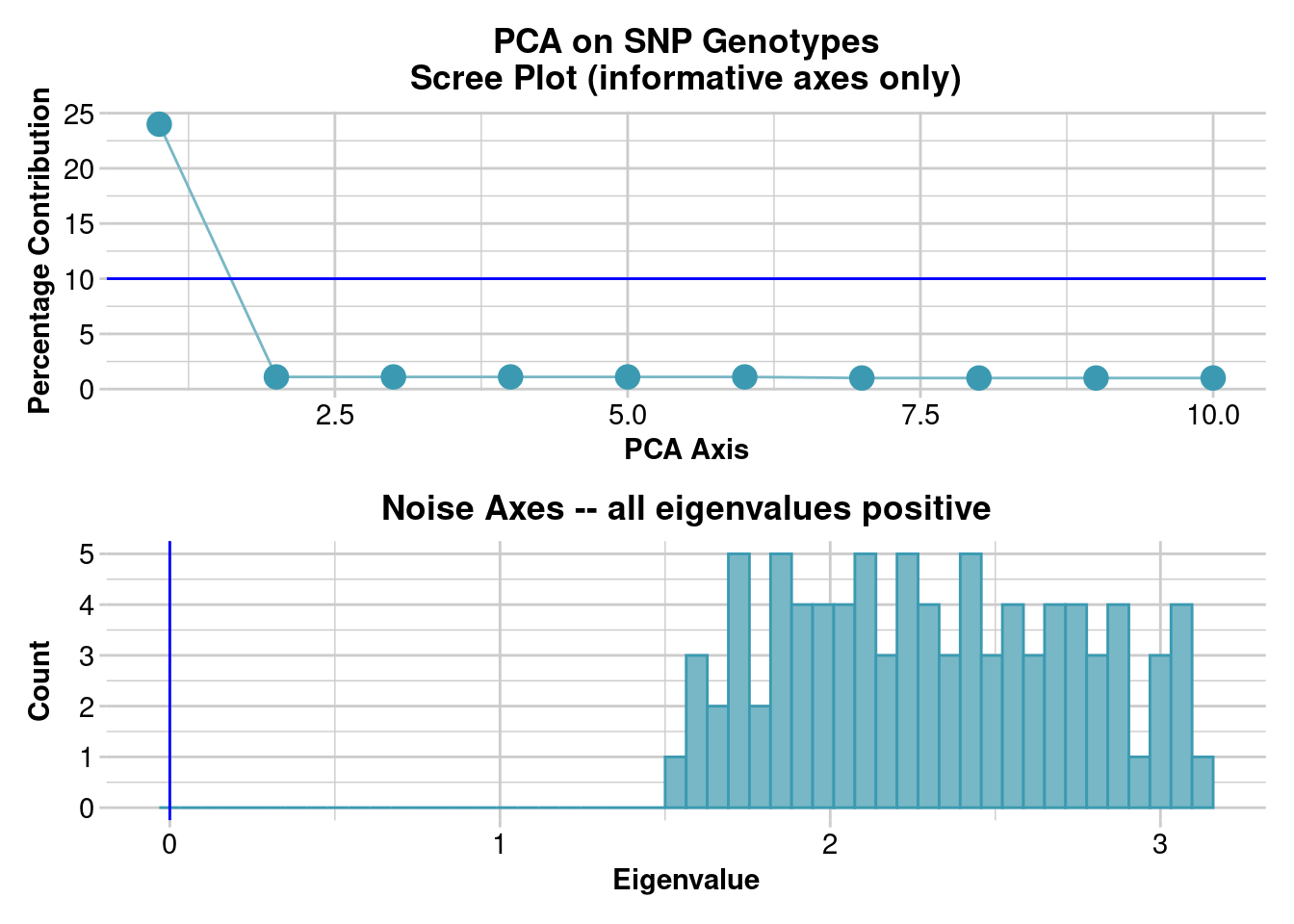 

Completed: gl.pcoa 

gl.pcoa.plot(glPca = pcaglsim, x = glsim)

Starting gl.pcoa.plot 
  Processing an ordination file (glPca)
  Processing genlight object with SNP data
Package directlabels  needed for this function to work. Please install it.

[1] -1

hwe <- gl.report.hwe(glsim, multi_comp = TRUE)

Starting gl.report.hwe 
  Processing genlight object with SNP data
Package HardyWeinberg  needed for this function to work. Please install it.

Assessing Populations: structure and demographic history

Load data and explore

This dataset is to assess population structure and diversity in Uperoleia crassa, from Jaya et al. (2022).

# gl <- dartR::gl.read.dart("Report_DUp20-4995_1_moreOrders_SNP_mapping_2.csv",
#                           ind.metafile = "Uperoleia_metadata.csv")

load('./data/session_2.RData') # data named gl

These are monsoonal tropical frogs, who are very common and abundant. They do evolutionarily and reproductively interesting and weird stuff.

Lets quickly look at our samples and populations.

gl.map.interactive(gl)

Starting gl.map.interactive 
  Processing genlight object with SNP data
Completed: gl.map.interactive 

We have two populations - the Kimberley (IK) and the Top End (IT)

Clean data

Clean up your dataset to remove the most egregiously bad loci and individuals this set of filtering can be used across analyses,

#Get rid of really poorly sequenced loci
#But don’t cut hard
gl.report.callrate(gl)

Starting gl.report.callrate 
  Processing genlight object with SNP data
  Reporting Call Rate by Locus
  No. of loci = 227143 
  No. of individuals = 36 
    Minimum      :  0.222222 
    1st quartile :  0.611111 
    Median       :  0.777778 
    Mean         :  0.7464089 
    3r quartile  :  0.916667 
    Maximum      :  1 
    Missing Rate Overall:  0.2536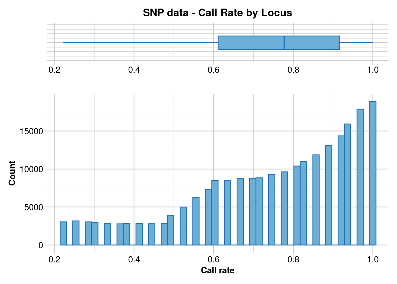 

Completed: gl.report.callrate 

gl.1 <- gl.filter.callrate(gl, method = "loc", threshold = 0.8)

Starting gl.filter.callrate 
  Processing genlight object with SNP data
  Warning: Data may include monomorphic loci in call rate 
                    calculations for filtering
  Recalculating Call Rate
  Removing loci based on Call Rate, threshold = 0.8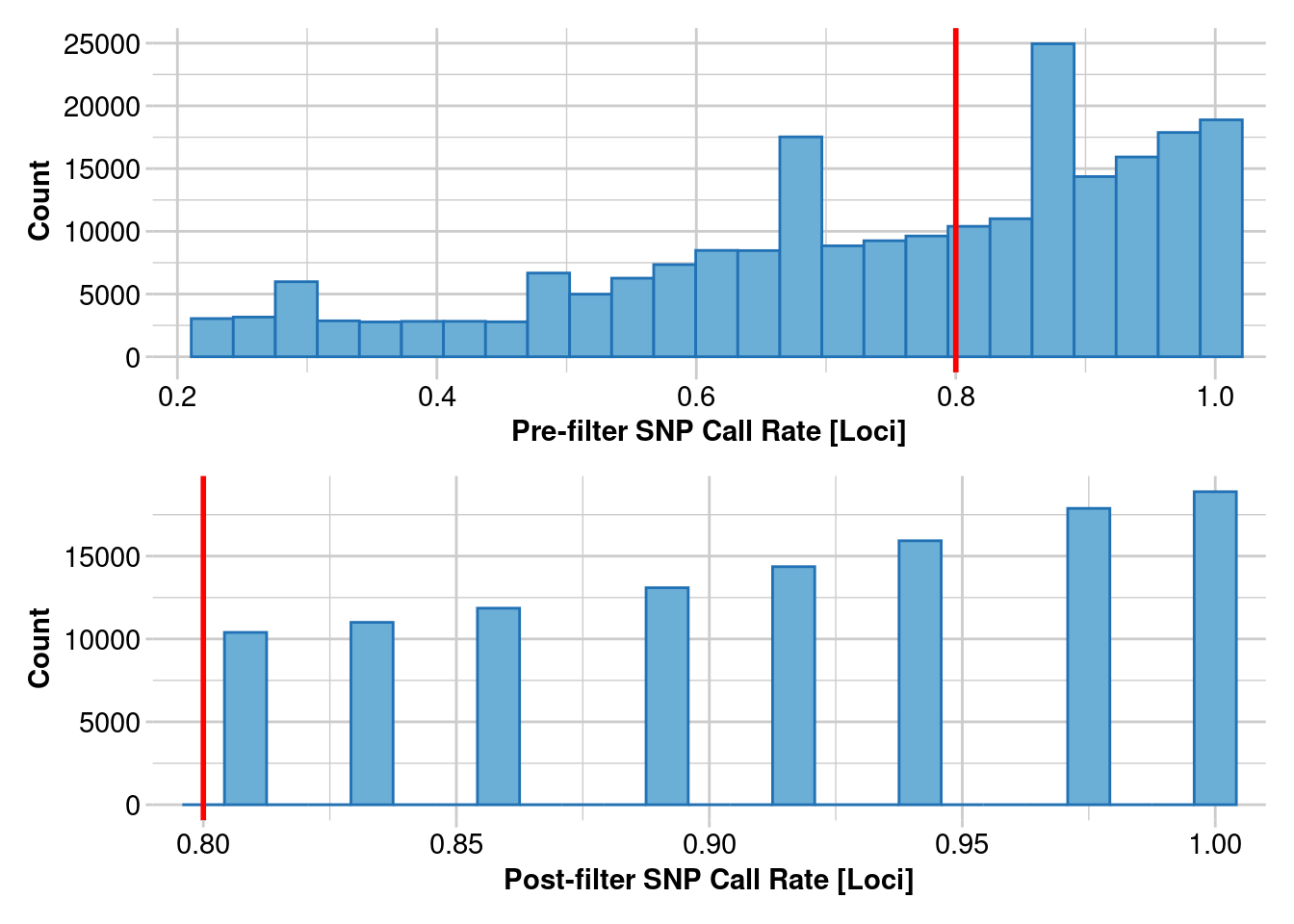 

Completed: gl.filter.callrate 

#Very low filter – this is only to get rid of your really bad individuals
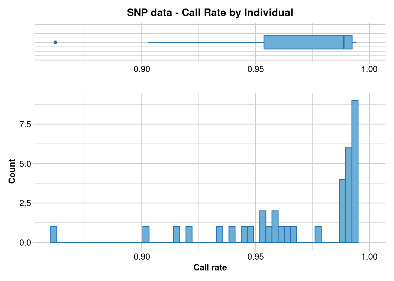
gl.report.callrate(gl.1, method = "ind")

Starting gl.report.callrate 
  Processing genlight object with SNP data

  Reporting Call Rate by Individual
  No. of loci = 113404 
  No. of individuals = 36 
    Minimum      :  0.7589944 
    1st quartile :  0.8751808 
    Median       :  0.9524179 
    Mean         :  0.9159171 
    3r quartile  :  0.9598625 
    Maximum      :  0.9787662 
    Missing Rate Overall:  0.0841 

Listing 2 populations and their average CallRates
  Monitor again after filtering
  Population CallRate  N
1         IK   0.9567 22
2         IT   0.8519 14

Listing 20 individuals with the lowest CallRates
  Use this list to see which individuals will be lost on filtering by individual
  Set ind.to.list parameter to see more individuals
          Individual  CallRate
1     Up1041_R138706 0.7589944
2    Up1186_QMJ88804 0.7730856
3      Up1096_R36195 0.8080932
4   Up0969_ABTC29129 0.8429597
5   Up1136_NTMR36228 0.8449878
6   Up0854_ABTC17229 0.8483299
7   Up0276_NTMR35114 0.8558869
8   Up1118_NTMR36173 0.8596699
9      Up1120_R36170 0.8701809
10  Up0767_ABTC12489 0.8768474
11  Up0731_ABTC99709 0.8850834
12  Up0832_ABTC93392 0.8948097
13  Up0769_ABTC12511 0.8980988
14 Up0166_WAMR162490 0.9082308
15     Up1078_R36177 0.9091390
16 Up1269_WAMR164857 0.9188212
17 Up1266_WAMR164844 0.9397640
18 Up1321_WAMR171536 0.9517389
19        WAMR162566 0.9530969
20 Up0083_WAMR113846 0.9537142

)

Completed: gl.report.callrate 

gl.2 <- gl.filter.callrate(gl.1, method = "ind", threshold = 0.25)

Starting gl.filter.callrate 
  Processing genlight object with SNP data
  Warning: Data may include monomorphic loci in call rate 
                    calculations for filtering
  Recalculating Call Rate
  Removing individuals based on Call Rate, threshold = 0.25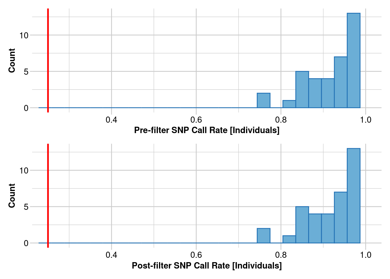 

  Note: Locus metrics not recalculated
  Note: Resultant monomorphic loci not deleted
Completed: gl.filter.callrate 

#Always run this after removing individuals – removes loci that are no longer variable
gl.3 <- gl.filter.monomorphs(gl.2)

Starting gl.filter.monomorphs 
  Processing genlight object with SNP data
  Identifying monomorphic loci
  No monomorphic loci to remove
Completed: gl.filter.monomorphs 

#Get rid of unreliable loci
gl.report.reproducibility(gl.3)

Starting gl.report.reproducibility 
  Processing genlight object with SNP data
  Reporting Repeatability by Locus
  No. of loci = 113404 
  No. of individuals = 36 
    Minimum      :  0.875 
    1st quartile :  1 
    Median       :  1 
    Mean         :  0.9962267 
    3r quartile  :  1 
    Maximum      :  1 
    Missing Rate Overall:  0.08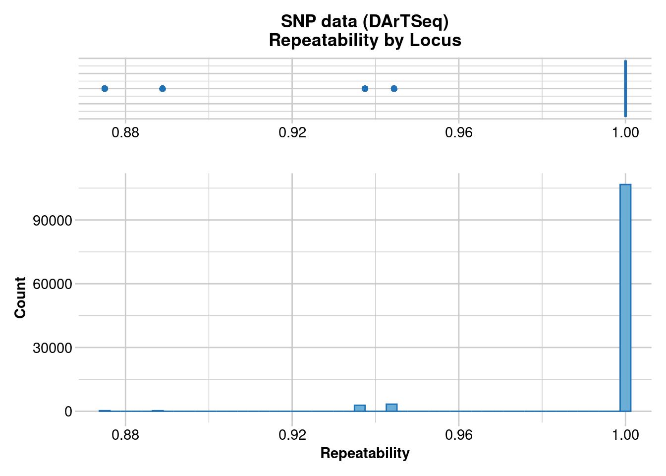 

   Quantile Threshold Retained Percent Filtered Percent
1      100%  1.000000   106676    94.1     6728     5.9
2       95%  1.000000   106676    94.1     6728     5.9
3       90%  1.000000   106676    94.1     6728     5.9
4       85%  1.000000   106676    94.1     6728     5.9
5       80%  1.000000   106676    94.1     6728     5.9
6       75%  1.000000   106676    94.1     6728     5.9
7       70%  1.000000   106676    94.1     6728     5.9
8       65%  1.000000   106676    94.1     6728     5.9
9       60%  1.000000   106676    94.1     6728     5.9
10      55%  1.000000   106676    94.1     6728     5.9
11      50%  1.000000   106676    94.1     6728     5.9
12      45%  1.000000   106676    94.1     6728     5.9
13      40%  1.000000   106676    94.1     6728     5.9
14      35%  1.000000   106676    94.1     6728     5.9
15      30%  1.000000   106676    94.1     6728     5.9
16      25%  1.000000   106676    94.1     6728     5.9
17      20%  1.000000   106676    94.1     6728     5.9
18      15%  1.000000   106676    94.1     6728     5.9
19      10%  1.000000   106676    94.1     6728     5.9
20       5%  0.944444   110021    97.0     3383     3.0
21       0%  0.875000   113404   100.0        0     0.0
Completed: gl.report.reproducibility 

gl.4 <- gl.filter.reproducibility(gl.3)

Starting gl.select.colors 
  Warning: Number of required colors not specified, set to 9
  Library: RColorBrewer
  Palette: brewer.pal
  Showing and returning 2 of 9 colors for library RColorBrewer : palette Blues 

Completed: gl.select.colors 
Starting gl.filter.reproducibility 
  Processing genlight object with SNP data
  Removing loci with repeatability less than 0.99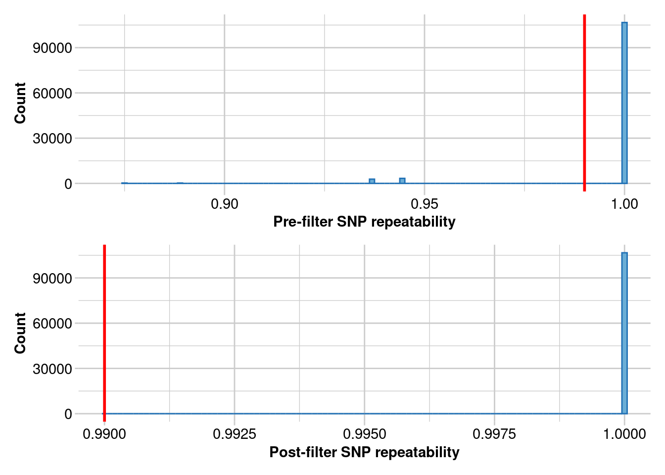 

Completed: gl.filter.reproducibility 

#Get rid of low and super high read depth loci
#do twice so you can zoom in
gl.report.rdepth(gl.4)

Starting gl.report.rdepth 
  Processing genlight object with SNP data
  Reporting Read Depth by Locus
  No. of loci = 106676 
  No. of individuals = 36 
    Minimum      :  2.5 
    1st quartile :  5 
    Median       :  7.2 
    Mean         :  7.741356 
    3r quartile  :  10 
    Maximum      :  121.7 
    Missing Rate Overall:  0.09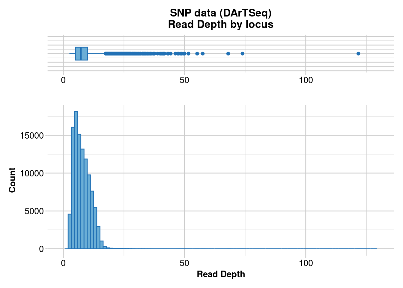 

   Quantile Threshold Retained Percent Filtered Percent
1      100%     121.7        1     0.0   106675   100.0
2       95%      13.6     5520     5.2   101156    94.8
3       90%      12.4    10872    10.2    95804    89.8
4       85%      11.5    16057    15.1    90619    84.9
5       80%      10.7    21633    20.3    85043    79.7
6       75%      10.0    26932    25.2    79744    74.8
7       70%       9.4    32193    30.2    74483    69.8
8       65%       8.8    37650    35.3    69026    64.7
9       60%       8.2    43461    40.7    63215    59.3
10      55%       7.7    48582    45.5    58094    54.5
11      50%       7.2    53911    50.5    52765    49.5
12      45%       6.7    59668    55.9    47008    44.1
13      40%       6.3    64353    60.3    42323    39.7
14      35%       5.8    70391    66.0    36285    34.0
15      30%       5.4    75457    70.7    31219    29.3
16      25%       5.0    80644    75.6    26032    24.4
17      20%       4.6    86041    80.7    20635    19.3
18      15%       4.2    91353    85.6    15323    14.4
19      10%       3.8    96433    90.4    10243     9.6
20       5%       3.3   102090    95.7     4586     4.3
21       0%       2.5   106676   100.0        0     0.0
Completed: gl.report.rdepth 

gl.5 <- gl.filter.rdepth(gl.4, lower = 0, upper = 25)

Starting gl.filter.rdepth 
  Processing genlight object with SNP data
  Removing loci with rdepth <= 0 and >= 25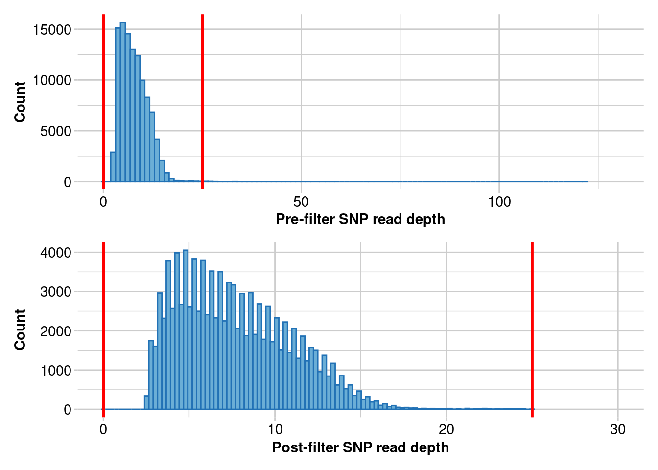 

Completed: gl.filter.rdepth 

gl.clean <- gl.filter.rdepth(gl.5, lower = 8, upper = 17)

Starting gl.filter.rdepth 
  Processing genlight object with SNP data
  Removing loci with rdepth <= 8 and >= 17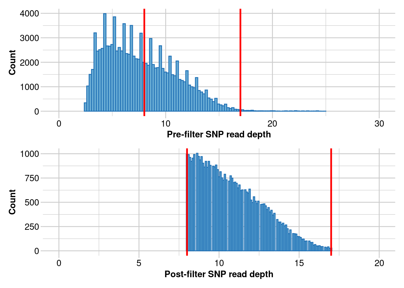 

Completed: gl.filter.rdepth 

nInd(gl.clean)

[1] 36

nLoc(gl.clean)

[1] 44752

#look at the data to see if you see any obvious issues and redo if you do.
plot(gl.clean)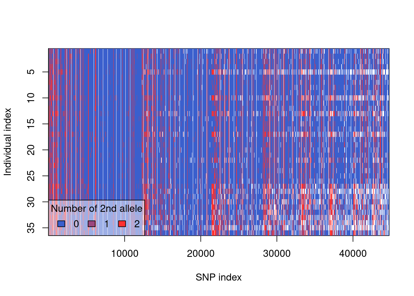

rm(gl.1, gl.2, gl.3, gl.4, gl.5)

gl.clean

This file is now your starting file for other filtering

Filtering

Filtering data for population structure and phylogenetic analyses

Loci on the same fragment and missing data are not well supported in these analyses, as they expect all loci to be independently inherited. This means very very close loci are not going to be split through recombination and should be removed. Structure-like analyses dislike missing data. We are also going to filter harder than normal here just so that we can see a result within the workshop.

gl.report.callrate(gl.clean)

gl.1 <- gl.filter.callrate(gl.clean, method = "loc", threshold = 0.98)

#Remove minor alleles
#I usually set up the threshold so it is just 
# removing singletons to improve computation time
gl.report.maf(gl.1)

gl.2 <- gl.filter.maf(gl.1,  threshold = 1/(2*nInd(gl.1)))

#check that the data looks fairly clean
#this starts to show some obvious population banding
plot(gl.2)

#remove secondary SNPs on the same fragment
#Always do this as the last loci filter so that you’ve cut for quality 
# before you cut because there are two SNPs
gl.3 <- gl.filter.secondaries(gl.2)

#Filter on individuals. You can usually be a bit flexible at this point.
#individuals look a whole lot better now
#make note of any idnviduals with a low call rate. Keep them in for now
#but if they act weird in the analysis, you may want to consider removing
gl.report.callrate(gl.3, method = "ind")

gl.4 <- gl.filter.callrate(gl.3, method = "ind", threshold = .9)

#Always run this after removing individuals
gl.structure <- gl.filter.monomorphs(gl.4)

#this is your cleaned dataset for a population structure analysis              
plot(gl.structure)

nInd(gl.structure)
nLoc(gl.structure)

You can write this file out for various analyses that we will not go into here (e.g. gl2structure(x) or gl2faststructure(x))

Run SNMF (LEA)

This is a structure-like analysis called SNMF. This code is not all you would need to publish this result, but it is a good first look. You need to test your parameter settings (alpha and tolerance) in a real analysis.

#takes quite a while to run (about 15 minutes)
#in case you want to run it uncomment the following lines and comment the readRDS line

# LEA requires the genotype style file
gl2faststructure(gl.structure, outfile = "gl_structure.fstr",
                outpath = './data/')
struct2geno("./data/gl_structure.fstr", ploidy = 2, FORMAT = 2)
###this hates any loci with all heterozygotes

snmf.Sy.K1_8.10 = snmf("./data/gl_structure.fstr.geno", K = 1:8,
                      entropy = T, ploidy = 2, project="new", repetitions = 10)

plot(snmf.Sy.K1_8.10)

k <- 2 #chose best based on lowest cross entropy in graph
ce = cross.entropy(snmf.Sy.K1_8.10, K = k)
best <- which.min(ce)
par (mfrow = c(1,1))
barplot(t(Q(snmf.Sy.K1_8.10, K = k, run = best)), col = 1:k)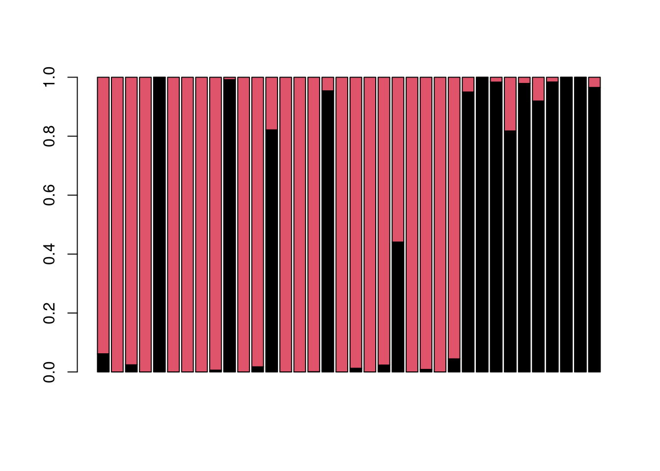

#Do a PCoA plot. I hate these but they are also good for first pass visualisation.
pc <- gl.pcoa(gl.structure)

Starting gl.pcoa 
  Processing genlight object with SNP data
  Performing a PCA, individuals as entities, loci as attributes, SNP genotype as state
Starting gl.colors 
Selected color type 2 
Completed: gl.colors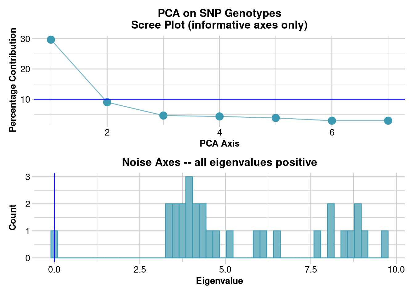 

Completed: gl.pcoa 

gl.pcoa.plot(pc, gl.structure)

Starting gl.pcoa.plot 
  Processing an ordination file (glPca)
  Processing genlight object with SNP data
Package directlabels  needed for this function to work. Please install it.

[1] -1

rm(ce, gl.1, gl.2, gl.3, gl.4, snmf.Sy.K1_8.10, best, k, pc)

Exercise

Have a go at altering various parameters and seeing how this changes your answers.

One thing that regularly changes with MAF filters is the amount of variance explained. Removing more minor alleles increases the variance explained in a PCoA. Think about why that would be the case.

Filtering for Tajima’s D

Now we are going to look at how filtering can affect your understanding of demographic processes that population is undergoing. In this case we are going to look at the metric Tajima’s D. Significant negative values of Tajima’s D are due to an excess of rare alleles and are consistent with range expansion. Significant positive values are associated with population contraction.

The moral of the story here is that rare alleles matter, especially when looking at population demographics! Lets look at how singletons impact our estimations of whether a population is expanding or contracting.

This is a function written to calculate Tajima’s D from SNP data. This code will create the function in your global environment so that you can call it. This function differs from calculations in packages such as heirfstat and popgen because it deals with missing data correctly for SNPs, while those other programs were built for gene alignments.Significance (a P-value) cannot be calculated without a simulation, and we are not doing that here. Please ask me how to do this using Hudson’s ms program if you are interested.

get_tajima_D <- function(x){
  #require(dartRverse) # possibly not needed for a function in an R package?
  
  # Find allele frequencies (p1 and p2) for every locus in every population
  allele_freqs <- dartR::gl.percent.freq(x)
  names(allele_freqs)[names(allele_freqs) == "frequency"] <- "p1"
  allele_freqs$p1 <- allele_freqs$p1 / 100
  allele_freqs$p2 <- 1 - allele_freqs$p1
  
  # Get the names of all the populations
  pops <- unique(allele_freqs$popn)
  
  #split each population
  allele_freqs_by_pop <- split(allele_freqs, allele_freqs$popn)
  
  # Internal function to calculate pi
  calc_pi <- function(allele_freqs) {
    n = allele_freqs$nobs * 2  # vector of n values
    pi_sqr <- allele_freqs$p1 ^ 2 + allele_freqs$p2 ^ 2
    h = (n / (n - 1)) * (1 - pi_sqr) # vector of values of h
    sum(h) # return pi, which is the sum of h across loci
  }
  
  get_tajima_D_for_one_pop <- function(allele_freqs_by_pop) {
    pi <- calc_pi(allele_freqs_by_pop)
    
# Calculate number of segregating sites, ignoring missing data (missing data will not appear in teh allele freq calcualtions)
    #S <- sum(!(allele_freqs_by_pop$p1 == 0 | allele_freqs_by_pop$p1 == 1))
    S <- sum(allele_freqs_by_pop$p1 >0 & allele_freqs_by_pop$p1 <1)
    if(S == 0) {
      warning("No segregating sites")
      data.frame(pi = NaN, 
                 S = NaN, 
                 D = NaN, 
                 Pval.normal = NaN, 
                 Pval.beta = NaN)
    }
    
    n <- mean(allele_freqs_by_pop$nobs * 2 )
    
    tmp <- 1:(n - 1)
    a1 <- sum(1/tmp)
    a2 <- sum(1/tmp^2)
    b1 <- (n + 1)/(3 * (n - 1))
    b2 <- 2 * (n^2 + n + 3)/(9 * n * (n - 1))
    c1 <- b1 - 1/a1
    c2 <- b2 - (n + 2)/(a1 * n) + a2/a1^2
    e1 <- c1/a1
    e2 <- c2/(a1^2 + a2)
    
    
    #calculate D and do beta testing
    D <- (pi - S/a1) / sqrt(e1 * S + e2 * S * (S - 1))
    Dmin <- (2/n - 1/a1)/sqrt(e2)
    Dmax <- ((n/(2*(n - 1))) - 1/a1)/sqrt(e2)
    tmp1 <- 1 + Dmin * Dmax
    tmp2 <- Dmax - Dmin
    a <- -tmp1 * Dmax/tmp2
    b <- tmp1 * Dmin/tmp2
  
    
    data.frame(pi = pi, 
               S = S, 
               D = D)
  }
  
  output <- do.call("rbind", lapply(allele_freqs_by_pop, 
                                    get_tajima_D_for_one_pop))
  data.frame(population = rownames(output), output, row.names = NULL)
}

We are going to focus on key filters and how they impact estimates

1. Minor allele frequency (MAF) filtering, which explicitly removes rare alleles

2. No MAF allele filtering and taking all data as it comes

3. No MAF filtering but filtering on read depth so we are confident in our rare alleles

1. MAF filtering

We will start with our lightly cleaned data and filter this for the tajima’s calculation.

#This function is written to calculate Tajima's D with a fair amount of missing data
#so we are going to filter lightly here
gl.report.callrate(gl.clean)

Starting gl.report.callrate 
  Processing genlight object with SNP data
  Reporting Call Rate by Locus
  No. of loci = 44752 
  No. of individuals = 36 
    Minimum      :  0.805556 
    1st quartile :  0.888889 
    Median       :  0.944444 
    Mean         :  0.9387004 
    3r quartile  :  1 
    Maximum      :  1 
    Missing Rate Overall:  0.0613 

Completed: gl.report.callrate 

gl.1 <- gl.filter.callrate(gl.clean, method = "loc", threshold = 0.9)

Starting gl.filter.callrate 
  Processing genlight object with SNP data
  Recalculating Call Rate
  Removing loci based on Call Rate, threshold = 0.9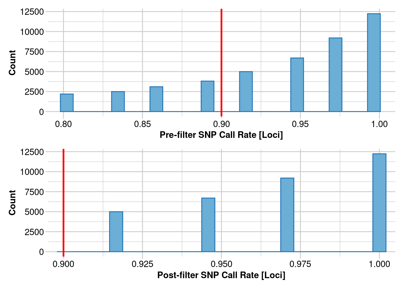 

Completed: gl.filter.callrate 

#In this first round, we are going to actually remove singletons (our rare alleles) to see what happens
gl.report.maf(gl.1)

Starting gl.report.maf 
  Processing genlight object with SNP data
Starting gl.report.maf 

  Reporting Minor Allele Frequency (MAF) by Locus for population IK 
  No. of loci = 14958 
  No. of individuals = 22 
    Minimum      :  0.0227 
    1st quantile :  0.0227 
    Median       :  0.0455 
    Mean         :  0.09433557 
    3r quantile  :  0.0952 
    Maximum      :  0.5 
    Missing Rate Overall:  0.01 

  Reporting Minor Allele Frequency (MAF) by Locus for population IT 
  No. of loci = 24122 
  No. of individuals = 14 
    Minimum      :  0.0357 
    1st quantile :  0.0385 
    Median       :  0.0769 
    Mean         :  0.1268348 
    3r quantile  :  0.1667 
    Maximum      :  0.5 
    Missing Rate Overall:  0.06 

  Reporting Minor Allele Frequency (MAF) by Locus OVERALL
  No. of loci = 33136 
  No. of individuals = 36 
    Minimum      :  0.0114 
    1st quantile :  0.0192 
    Median       :  0.0384 
    Mean         :  0.08512636 
    3r quantile  :  0.0893 
    Maximum      :  0.5 
    Missing Rate Overall:  0.03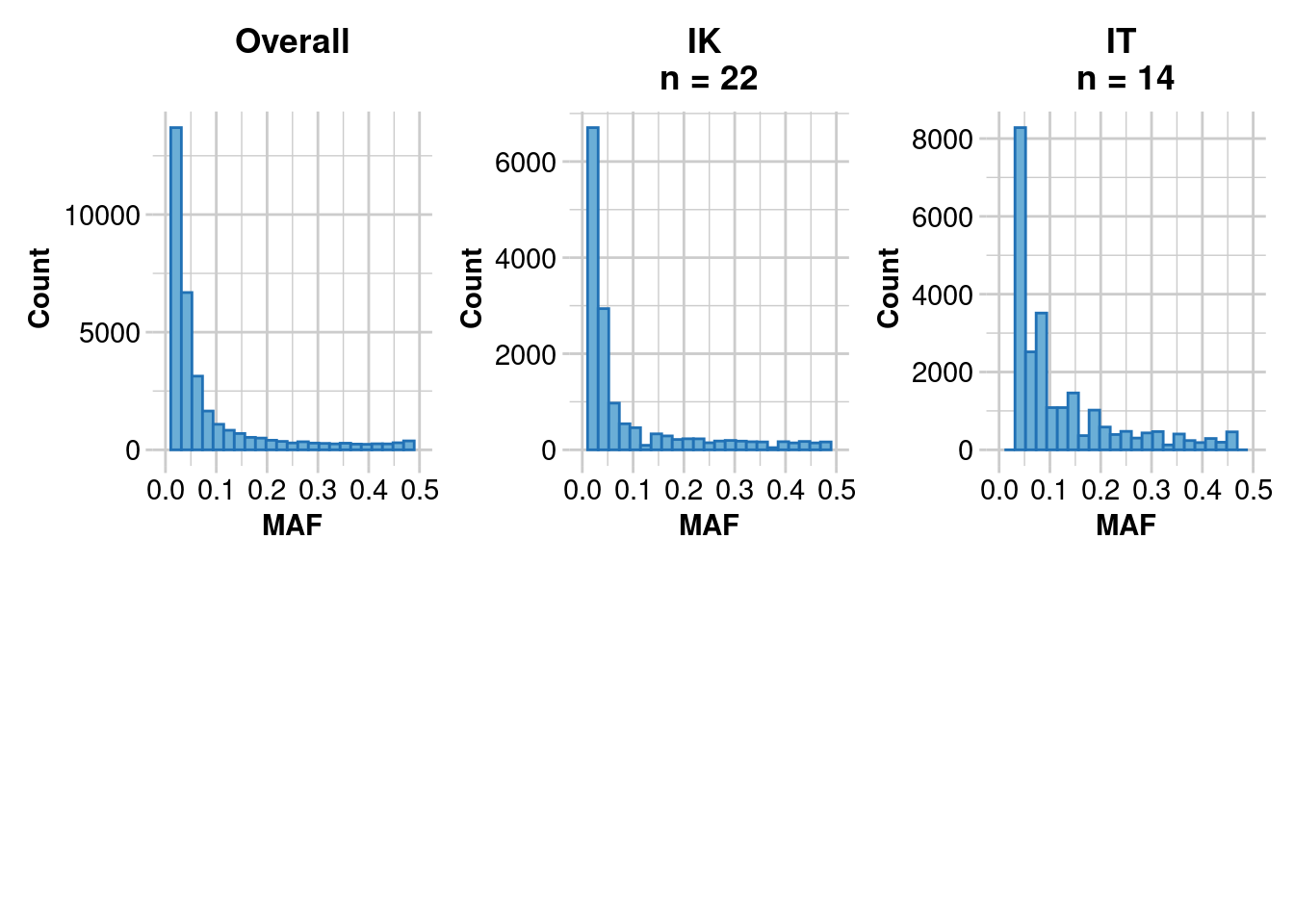 

   Quantile Threshold Retained Percent Filtered Percent
1      100%    0.5000       75     0.2    33061    99.8
2       95%    0.3785     1657     5.0    31479    95.0
3       90%    0.2559     3314    10.0    29822    90.0
4       85%    0.1705     4984    15.0    28152    85.0
5       80%    0.1190     6630    20.0    26506    80.0
6       75%    0.0893     8533    25.8    24603    74.2
7       70%    0.0714    10159    30.7    22977    69.3
8       65%    0.0577    11608    35.0    21528    65.0
9       60%    0.0454    13989    42.2    19147    57.8
10      55%    0.0416    15067    45.5    18069    54.5
11      50%    0.0384    16598    50.1    16538    49.9
12      45%    0.0357    18691    56.4    14445    43.6
13      40%    0.0292    19887    60.0    13249    40.0
14      35%    0.0227    22254    67.2    10882    32.8
15      30%    0.0209    23242    70.1     9894    29.9
16      25%    0.0192    25099    75.7     8037    24.3
17      20%    0.0178    28849    87.1     4287    12.9
18      15%    0.0178    28849    87.1     4287    12.9
19      10%    0.0114    32776    98.9      360     1.1
20       5%    0.0114    32776    98.9      360     1.1
21       0%    0.0114    33136   100.0        0     0.0
Completed: gl.report.maf 

nLoc(gl.1)

[1] 33136

gl.2 <- gl.filter.maf(gl.1,  threshold = 0.05)

Starting gl.select.colors 
  Warning: Number of required colors not specified, set to 9
  Library: RColorBrewer
  Palette: brewer.pal
  Showing and returning 2 of 9 colors for library RColorBrewer : palette Blues 

Completed: gl.select.colors 
Starting gl.filter.maf 
  Processing genlight object with SNP data
  Removing loci with MAF < 0.05 over all the dataset 
                and recalculating FreqHoms and FreqHets

Completed: gl.filter.maf 

nLoc(gl.2)

[1] 12823

#check that the data looks fairly clean
#this starts to show some obvious banding which are the two populations
plot(gl.2)

#we are also going to remove secondary SNPs on the same fragment in this first round
gl.3 <- gl.filter.secondaries(gl.2)

Starting gl.filter.secondaries 
  Processing genlight object with SNP data
  Selecting one SNP per sequence tag at random
Completed: gl.filter.secondaries 

#Filter on individuals. You can usually be a bit flexible at this point.
#make note of any individuals with a low call rate. Keep them in for now
#but if they act weird in the analysis, you may want to consider removing
gl.report.callrate(gl.3, method = "ind")

Starting gl.report.callrate 
  Processing genlight object with SNP data

  Reporting Call Rate by Individual
  No. of loci = 10422 
  No. of individuals = 36 
    Minimum      :  0.8513721 
    1st quartile :  0.9509211 
    Median       :  0.9869507 
    Mean         :  0.9658255 
    3r quartile  :  0.9918922 
    Maximum      :  0.9948187 
    Missing Rate Overall:  0.0342 

Listing 2 populations and their average CallRates
  Monitor again after filtering
  Population CallRate  N
1         IK   0.9878 22
2         IT   0.9313 14

Listing 20 individuals with the lowest CallRates
  Use this list to see which individuals will be lost on filtering by individual
  Set ind.to.list parameter to see more individuals
          Individual  CallRate
1     Up1041_R138706 0.8513721
2    Up1186_QMJ88804 0.8919593
3      Up1096_R36195 0.9030896
4   Up0854_ABTC17229 0.9175782
5   Up0969_ABTC29129 0.9260219
6      Up1120_R36170 0.9375360
7   Up1118_NTMR36173 0.9396469
8   Up0767_ABTC12489 0.9418538
9   Up0832_ABTC93392 0.9507772
10  Up0731_ABTC99709 0.9509691
11  Up1136_NTMR36228 0.9531760
12  Up0769_ABTC12511 0.9537517
13 Up1269_WAMR164857 0.9573019
14  Up0276_NTMR35114 0.9580695
15     Up1078_R36177 0.9618116
16 Up0166_WAMR162490 0.9654577
17 Up1266_WAMR164844 0.9762042
18 Up0183_WAMR162558 0.9866628
19 Up1321_WAMR171536 0.9872385
20        WAMR162566 0.9877183

)

Completed: gl.report.callrate 

gl.4 <- gl.filter.callrate(gl.3, method = "ind", threshold = .9)

Starting gl.filter.callrate 
  Processing genlight object with SNP data
  Recalculating Call Rate
  Removing individuals based on Call Rate, threshold = 0.9 
  Individuals deleted (CallRate <=  0.9 ):
Up1186_QMJ88804[IT], Up1041_R138706[IT],

  Note: Locus metrics not recalculated
  Note: Resultant monomorphic loci not deleted
Completed: gl.filter.callrate 

#Always run this after removing individuals
gl.D_withfiltering <- gl.filter.monomorphs(gl.4)

Starting gl.filter.monomorphs 
  Processing genlight object with SNP data
  Identifying monomorphic loci
  Removing monomorphic loci and loci with all missing 
                       data
Completed: gl.filter.monomorphs 

#calculate tajima's D with removing singletons and secondaries
gl.D_withfiltering

 ********************
 *** DARTR OBJECT ***
 ********************

 ** 34 genotypes,  9,857 SNPs , size: 70.6 Mb

    missing data: 9571 (=2.86 %) scored as NA

 ** Genetic data
   @gen: list of 34 SNPbin
   @ploidy: ploidy of each individual  (range: 2-2)

 ** Additional data
   @ind.names:  34 individual labels
   @loc.names:  9857 locus labels
   @loc.all:  9857 allele labels
   @position: integer storing positions of the SNPs [within 69 base sequence]
   @pop: population of each individual (group size range: 12-22)
   @other: a list containing: loc.metrics, ind.metrics, latlon, loc.metrics.flags, verbose, history 
    @other$ind.metrics: id, pop, popx, lat, lon, service, plate_location 
    @other$loc.metrics: AlleleID, CloneID, AlleleSequence, TrimmedSequence, SNP, SnpPosition, CallRate, OneRatioRef, OneRatioSnp, FreqHomRef, FreqHomSnp, FreqHets, PICRef, PICSnp, AvgPIC, AvgCountRef, AvgCountSnp, RepAvg, clone, uid, rdepth, maf 
   @other$latlon[g]: coordinates for all individuals are attached

D_w_filtering <- get_tajima_D(gl.D_withfiltering)

Registered S3 method overwritten by 'GGally':
  method from   
  +.gg   ggplot2

Registered S3 method overwritten by 'genetics':
  method      from 
  [.haplotype pegas

Registered S3 methods overwritten by 'dartR':
  method      from      
  cbind.dartR dartR.base
  rbind.dartR dartR.base

Starting :: 
 Starting dartR 
 Starting gl.percent.freq 
  Processing genlight object with SNP data
Starting gl.percent.freq: Calculating allele frequencies for populations
Completed: :: 
 Completed: dartR 
 Completed: gl.percent.freq 

D_w_filtering

  population        pi    S          D
1         IK  729.9187 4809 -1.2812312
2         IT 1511.4575 6863 -0.8129841

rm(gl.1, gl.2, gl.3, gl.4)

2. No MAF filtering

Now lets try it where we don’t remove singletons or secondaries

#This function is written to calculate Tajima's D with a fair amount of missing data
#we are going to filter lightly here 
gl.report.callrate(gl.clean)

Starting gl.report.callrate 
  Processing genlight object with SNP data
  Reporting Call Rate by Locus
  No. of loci = 44752 
  No. of individuals = 36 
    Minimum      :  0.805556 
    1st quartile :  0.888889 
    Median       :  0.944444 
    Mean         :  0.9387004 
    3r quartile  :  1 
    Maximum      :  1 
    Missing Rate Overall:  0.0613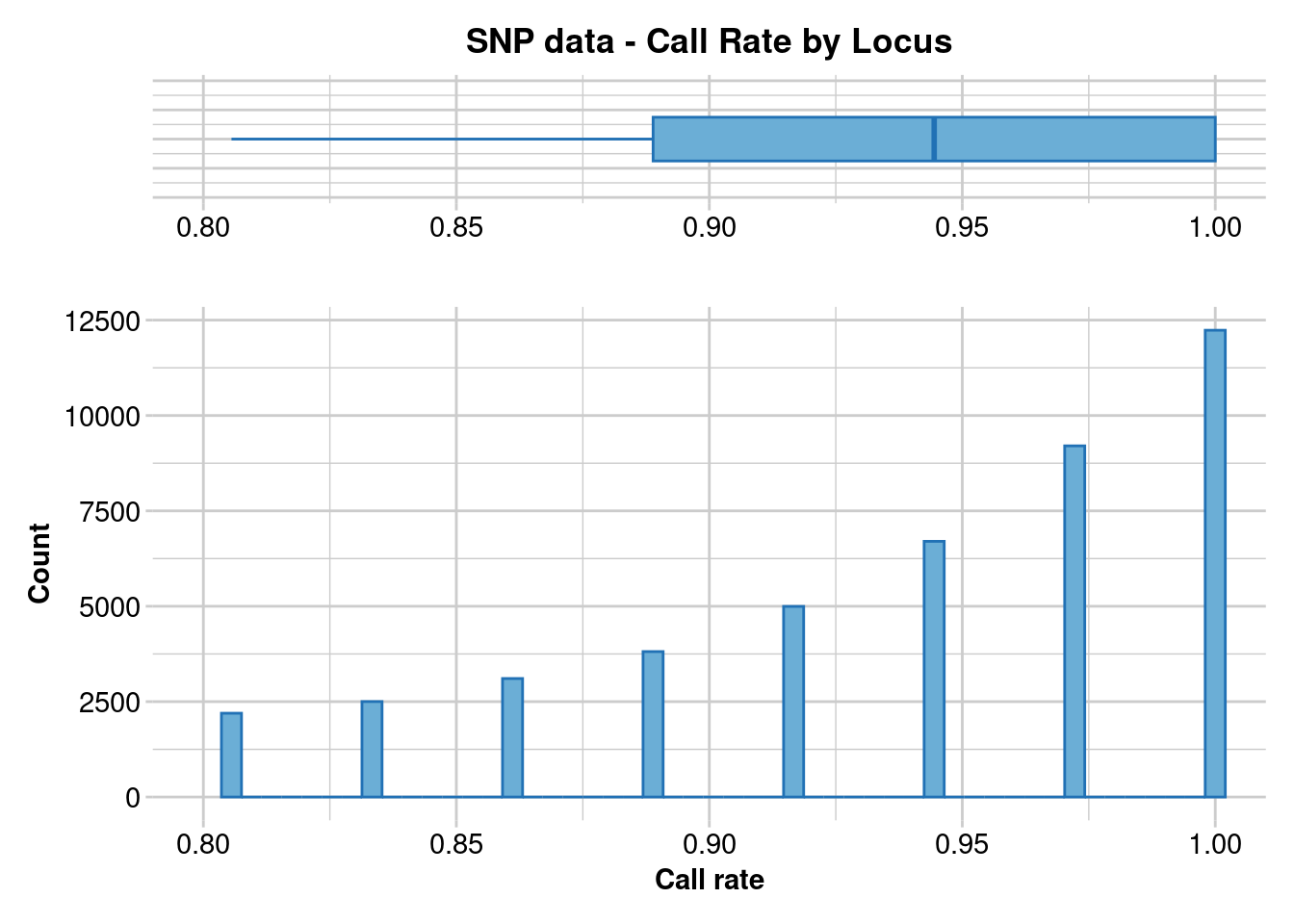 

Completed: gl.report.callrate 

gl.1 <- gl.filter.callrate(gl.clean, method = "loc", threshold = 0.9)

Starting gl.filter.callrate 
  Processing genlight object with SNP data
  Recalculating Call Rate
  Removing loci based on Call Rate, threshold = 0.9 

Completed: gl.filter.callrate 

#check that the data looks fairly clean
#this starts ot show some obvious population banding
plot(gl.1)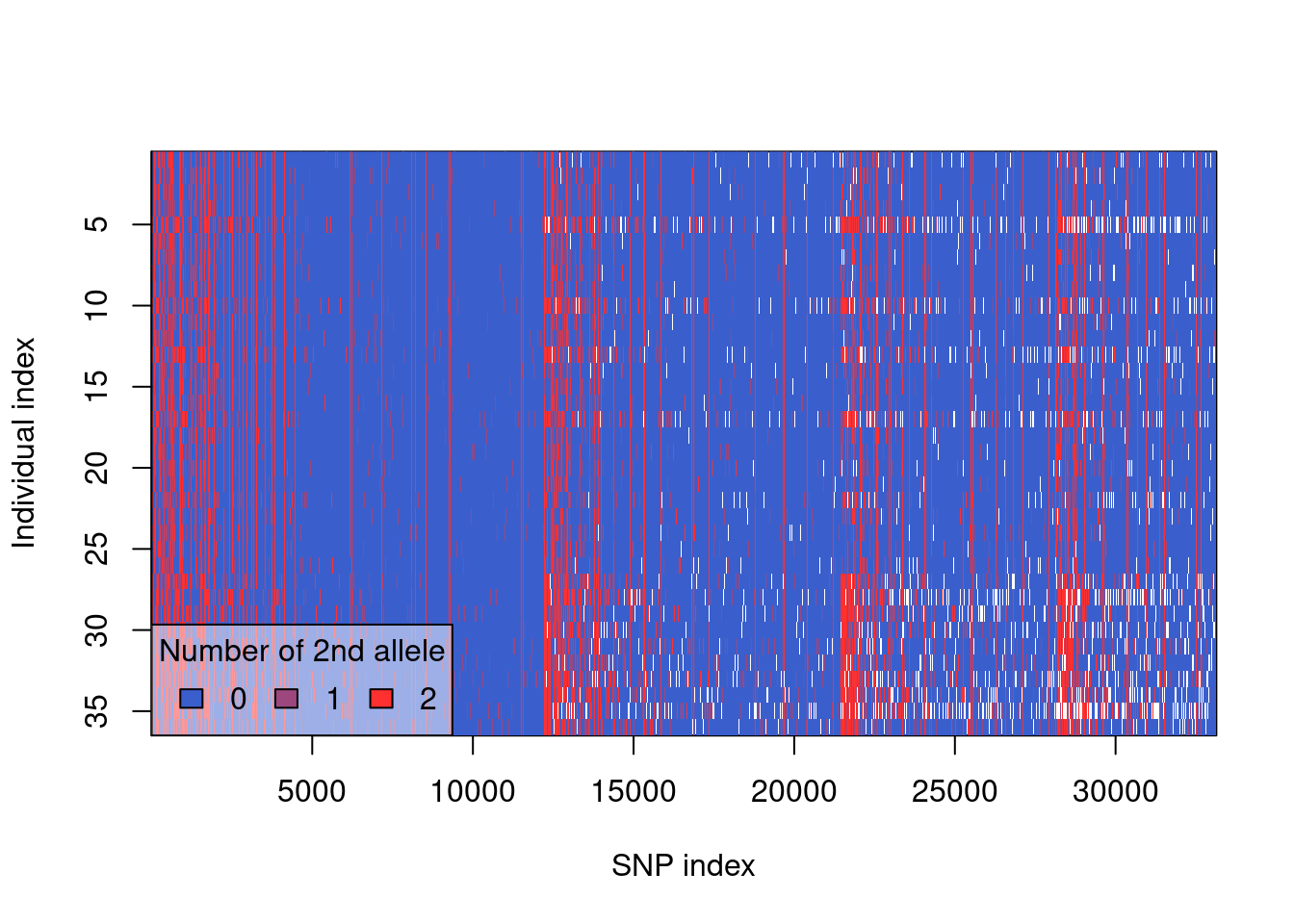

#Filter on individuals. You can usually be a bit flexible at this point.
#make note of any idnviduals with a low call rate. Keep them in for now
#but if they act weird in the analysis, you may want to consider removing
gl.report.callrate(gl.1, method = "ind")

Starting gl.report.callrate 
  Processing genlight object with SNP data

  Reporting Call Rate by Individual
  No. of loci = 33136 
  No. of individuals = 36 
    Minimum      :  0.8620232 
    1st quartile :  0.9536758 
    Median       :  0.9886679 
    Mean         :  0.9684834 
    3r quartile  :  0.9923648 
    Maximum      :  0.9943264 
    Missing Rate Overall:  0.0315 

Listing 2 populations and their average CallRates
  Monitor again after filtering
  Population CallRate  N
1         IK   0.9888 22
2         IT   0.9366 14

Listing 20 individuals with the lowest CallRates
  Use this list to see which individuals will be lost on filtering by individual
  Set ind.to.list parameter to see more individuals
          Individual  CallRate
1     Up1041_R138706 0.8620232
2    Up1186_QMJ88804 0.9028549
3      Up1096_R36195 0.9145039
4   Up0854_ABTC17229 0.9209319
5   Up0969_ABTC29129 0.9341803
6      Up1120_R36170 0.9400954
7   Up1118_NTMR36173 0.9462216
8   Up0767_ABTC12489 0.9478211
9   Up0731_ABTC99709 0.9527704
10  Up1136_NTMR36228 0.9539775
11  Up0832_ABTC93392 0.9551545
12  Up0276_NTMR35114 0.9586251
13  Up0769_ABTC12511 0.9594097
14 Up1269_WAMR164857 0.9621861
15     Up1078_R36177 0.9633028
16 Up0166_WAMR162490 0.9667733
17 Up1266_WAMR164844 0.9783317
18 Up1321_WAMR171536 0.9882001
19 Up0083_WAMR113846 0.9891357
20 Up0183_WAMR162558 0.9891960

)

Completed: gl.report.callrate 

gl.2 <- gl.filter.callrate(gl.1, method = "ind", threshold = .9)

Starting gl.filter.callrate 
  Processing genlight object with SNP data
  Recalculating Call Rate
  Removing individuals based on Call Rate, threshold = 0.9 
  Individuals deleted (CallRate <=  0.9 ):
Up1041_R138706[IT],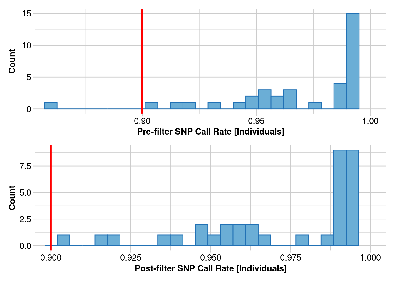

  Note: Locus metrics not recalculated
  Note: Resultant monomorphic loci not deleted
Completed: gl.filter.callrate 

#Always run this after removing individuals
gl.D_withOutfiltering <- gl.filter.monomorphs(gl.2)

Starting gl.filter.monomorphs 
  Processing genlight object with SNP data
  Identifying monomorphic loci
  Removing monomorphic loci and loci with all missing 
                       data
Completed: gl.filter.monomorphs 

rm(gl.1, gl.2)

D_wOUT_filtering <- get_tajima_D(gl.D_withOutfiltering)

Starting :: 
 Starting dartR 
 Starting gl.percent.freq 
  Processing genlight object with SNP data
Starting gl.percent.freq: Calculating allele frequencies for populations
Completed: :: 
 Completed: dartR 
 Completed: gl.percent.freq 

3. No MAF filtering but filtering on Read depth

Now lets try it where we don’t remove singletons or secondaries AND we filter for read depth to remove singletons where we are not confident about their base calls

#This function is written to calculate Tajima's D with a fair amount of missing data
# we are going to filter lightly here 
gl.report.callrate(gl.clean)

Starting gl.report.callrate 
  Processing genlight object with SNP data
  Reporting Call Rate by Locus
  No. of loci = 44752 
  No. of individuals = 36 
    Minimum      :  0.805556 
    1st quartile :  0.888889 
    Median       :  0.944444 
    Mean         :  0.9387004 
    3r quartile  :  1 
    Maximum      :  1 
    Missing Rate Overall:  0.0613 

Completed: gl.report.callrate 

gl.1 <- gl.filter.callrate(gl.clean, method = "loc", threshold = 0.9)

Starting gl.filter.callrate 
  Processing genlight object with SNP data
  Recalculating Call Rate
  Removing loci based on Call Rate, threshold = 0.9 

Completed: gl.filter.callrate 

#check that the data looks fairly clean
#this starts ot show some obvious population banding
plot(gl.1)

#filter to loci with a lower read depth, so that we are really confident
#that our base calls are correct
gl.report.rdepth(gl.1)

Starting gl.report.rdepth 
  Processing genlight object with SNP data
  Reporting Read Depth by Locus
  No. of loci = 33136 
  No. of individuals = 36 
    Minimum      :  8 
    1st quartile :  9.3 
    Median       :  10.7 
    Mean         :  10.94332 
    3r quartile  :  12.4 
    Maximum      :  17 
    Missing Rate Overall:  0.03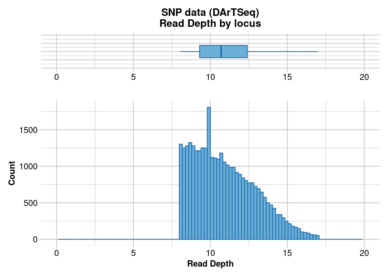 

   Quantile Threshold Retained Percent Filtered Percent
1      100%      17.0       27     0.1    33109    99.9
2       95%      14.7     1707     5.2    31429    94.8
3       90%      13.8     3536    10.7    29600    89.3
4       85%      13.3     5002    15.1    28134    84.9
5       80%      12.8     6811    20.6    26325    79.4
6       75%      12.4     8369    25.3    24767    74.7
7       70%      12.0    10014    30.2    23122    69.8
8       65%      11.6    11913    36.0    21223    64.0
9       60%      11.3    13385    40.4    19751    59.6
10      55%      11.0    14934    45.1    18202    54.9
11      50%      10.7    16641    50.2    16495    49.8
12      45%      10.4    18337    55.3    14799    44.7
13      40%      10.1    19974    60.3    13162    39.7
14      35%       9.8    21780    65.7    11356    34.3
15      30%       9.5    23645    71.4     9491    28.6
16      25%       9.3    24859    75.0     8277    25.0
17      20%       9.0    26704    80.6     6432    19.4
18      15%       8.7    28644    86.4     4492    13.6
19      10%       8.5    29974    90.5     3162     9.5
20       5%       8.2    31834    96.1     1302     3.9
21       0%       8.0    33136   100.0        0     0.0
Completed: gl.report.rdepth 

gl.2 <- gl.filter.rdepth(gl.1, lower = 12, upper = 17)

Starting gl.filter.rdepth 
  Processing genlight object with SNP data
  Removing loci with rdepth <= 12 and >= 17 

Completed: gl.filter.rdepth 

#Filter on individuals. You can usually be a bit flexible at this point.
#make note of any idnviduals with a low call rate. Keep them in for now
#but if they act weird in the analysis, you may want to consider removing
gl.report.callrate(gl.2, method = "ind")

Starting gl.report.callrate 
  Processing genlight object with SNP data

  Reporting Call Rate by Individual
  No. of loci = 10014 
  No. of individuals = 36 
    Minimum      :  0.8722788 
    1st quartile :  0.9646245 
    Median       :  0.9926103 
    Mean         :  0.9749822 
    3r quartile  :  0.9955063 
    Maximum      :  0.9969043 
    Missing Rate Overall:  0.025 

Listing 2 populations and their average CallRates
  Monitor again after filtering
  Population CallRate  N
1         IK   0.9926 22
2         IT   0.9473 14

Listing 20 individuals with the lowest CallRates
  Use this list to see which individuals will be lost on filtering by individual
  Set ind.to.list parameter to see more individuals
          Individual  CallRate
1     Up1041_R138706 0.8722788
2    Up1186_QMJ88804 0.9191132
3      Up1096_R36195 0.9281007
4   Up0854_ABTC17229 0.9320951
5   Up0969_ABTC29129 0.9398842
6      Up1120_R36170 0.9531656
7   Up1118_NTMR36173 0.9573597
8   Up0767_ABTC12489 0.9620531
9   Up0832_ABTC93392 0.9636509
10     Up1078_R36177 0.9649491
11  Up0731_ABTC99709 0.9657480
12  Up0769_ABTC12511 0.9662473
13  Up1136_NTMR36228 0.9678450
14  Up0276_NTMR35114 0.9690433
15 Up1269_WAMR164857 0.9721390
16 Up0166_WAMR162490 0.9740363
17 Up1266_WAMR164844 0.9870182
18 Up1321_WAMR171536 0.9924106
19        WAMR162566 0.9928101
20 Up0183_WAMR162558 0.9928101

)

Completed: gl.report.callrate 

gl.3 <- gl.filter.callrate(gl.2, method = "ind", threshold = .9)

Starting gl.filter.callrate 
  Processing genlight object with SNP data
  Recalculating Call Rate
  Removing individuals based on Call Rate, threshold = 0.9 
  Individuals deleted (CallRate <=  0.9 ):
Up1041_R138706[IT],

  Note: Locus metrics not recalculated
  Note: Resultant monomorphic loci not deleted
Completed: gl.filter.callrate 

#Always run this after removing individuals
gl.D_withOutfilteringRDepth <- gl.filter.monomorphs(gl.3)

Starting gl.filter.monomorphs 
  Processing genlight object with SNP data
  Identifying monomorphic loci
  Removing monomorphic loci and loci with all missing 
                       data
Completed: gl.filter.monomorphs 

rm(gl.1, gl.2, gl.3)

#calculate tajima's D with removing singletons and secondaries

D_wOUT_filtering_Rdepth <- get_tajima_D(gl.D_withOutfilteringRDepth)

Starting :: 
 Starting dartR 
 Starting gl.percent.freq 
  Processing genlight object with SNP data
Starting gl.percent.freq: Calculating allele frequencies for populations
Completed: :: 
 Completed: dartR 
 Completed: gl.percent.freq 

Results

lets look at all three

D_w_filtering

  population        pi    S          D
1         IK  729.9187 4809 -1.2812312
2         IT 1511.4575 6863 -0.8129841

D_wOUT_filtering

  population       pi     S          D
1         IK 2191.305 14958 -1.3671682
2         IT 4788.202 22787 -0.8746524

D_wOUT_filtering_Rdepth

  population        pi    S          D
1         IK  674.2647 4643 -1.3871722
2         IT 1494.1162 6981 -0.8153518

Interpreting results

For our Kimberley population, removing minor alleles give the actual wrong answer and suggests the population is contracting. This would have contradicted the rest of the findings of the paper, and been an artifact of the filtering process.

This shows how understanding the population genetic theory for a metric is crucial to useful analyses.

Further Study

Another teaching app in R, covering only Shannon for genes and its change over time, produced by Computer Science and Engineering third-year students: https://evolutionaryecology.shinyapps.io/learningEE

Readings

O’Reilly et al. (2020)

Sherwin (2022)

Sherwin et al. (2017)

Sherwin et al. (2021)

Jaya et al. (2022)

Jaya, Frederick R., Jessie C. Tanner, Michael R. Whitehead, Paul Doughty, J. Scott Keogh, Craig C. Moritz, and Renee A. Catullo. 2022. “Population Genomics and Sexual Signals Support Reproductive Character Displacement in Uperoleia (Anura: Myobatrachidae) in a Contact Zone.” Molecular Ecology 31 (17): 4527–43. https://doi.org/10.1111/mec.16597.

O’Reilly, G. D., F. Jabot, M. R. Gunn, and W. B. Sherwin. 2020. “Predicting Shannon’s Information for Genes in Finite Populations: New Uses for Old Equations.” Conservation Genetics Resources 12 (2): 245–55. https://doi.org/10.1007/s12686-018-1079-z.

Sherwin, W. B. 2022. “Bray-Curtis (AFD) Differentiation in Molecular Ecology: Forecasting, an Adjustment (AA), and Comparative Performance in Selection Detection.” Ecology and Evolution 12 (9): e9176. https://doi.org/10.1002/ece3.9176.

Sherwin, W. B., A. Chao, L. Jost, and P. E. Smouse. 2017. “Information Theory Broadens the Spectrum of Molecular Ecology and Evolution.” Trends in Ecology & Evolution 32 (12): 948–63. https://doi.org/10.1016/j.tree.2017.09.012.

———. 2021. “Information Theory Broadens the Spectrum of Molecular Ecology and Evolution: (Trends in Ecology and Evolution 32:12, p:948–963, 2017).” Trends in Ecology & Evolution 36 (10): 955–56. https://doi.org/10.1016/j.tree.2021.07.005.